Gold is one of the most actively monitored financial instruments in the global market. Its price, commonly represented by the XAUUSD trading pair, expresses the value of gold relative to the US dollar. Gold price movements can be influenced by monetary policy, inflation expectations, currency fluctuations, geopolitical uncertainty, and changes in investor sentiment. These characteristics make XAUUSD an interesting instrument for technical analysis and trading strategy development.

Technical analysis uses historical price information and mathematical indicators to examine market trends, momentum, volatility, and potential price boundaries. Several widely used indicators include the Simple Moving Average (SMA), Relative Strength Index (RSI), Moving Average Convergence Divergence (MACD), and Bollinger Bands. Although each indicator provides different information, combining them can help establish a more structured framework for evaluating market conditions.

Python provides an effective environment for developing automated financial analysis systems. Through libraries such as Requests, Pandas, NumPy, and Matplotlib, historical market data can be retrieved, processed, analyzed, and visualized within a single workflow. Furthermore, historical backtesting can be used to investigate how a predefined trading strategy would have performed on past price data.

This article develops a Python-based analytical framework for XAUUSD using the MarketFlow All-in-One Market Finance API. The framework consists of five main computational cells covering API configuration, market data retrieval, technical indicator calculation, trading signal generation, visualization, and historical backtesting.

The primary objective is to demonstrate an integrated and reproducible workflow for technical market analysis. The resulting framework is intended as an analytical tool for examining trading conditions rather than a guarantee of future profitability.

Methodology

The methodology consists of five sequential computational stages. Each stage performs a specific task and provides the data required by the subsequent stage.

The first stage initializes the Python environment and configures API authentication. The second retrieves market information and historical price data. The third processes the retrieved candlestick records and calculates technical indicators. The fourth generates potential trading signals and visualizes the resulting indicators. Finally, the fifth evaluates a basic trading strategy using historical returns and risk metrics.

The implementation uses the daily XAUUSD timeframe, with a requested historical range of 500 candles. The actual number of observations depends on the data returned by the API and the data-cleaning process.

Cell 1 — API Configuration and Market Discovery

The first computational cell establishes the Python environment and initializes the connection to the MarketFlow API. The Requests library provides HTTP communication, Pandas handles market datasets, NumPy supports numerical operations, and Matplotlib supplies visualization capabilities.

API authentication is managed through a RapidAPI key. The program first attempts to retrieve the key from the RAPIDAPI_KEY environment variable. If the variable is unavailable, the getpass function requests the key interactively. This approach reduces the need to store authentication credentials directly in the source code.

A reusable api_get() function sends authenticated GET requests, applies a 30-second timeout, checks the HTTP response status, and returns the response as JSON data. This function centralizes API communication and makes subsequent requests easier to manage.

The configuration defines the target instrument as OANDA:XAUUSD, the daily timeframe as D, the requested candle range as 500, and the timezone as Asia/Jakarta. These parameters establish the initial settings for the analysis.

Code — Cell 1

%pip -q install requests pandas numpy matplotlib

import os
import getpass
import requests
import numpy as np
import pandas as pd
import matplotlib.pyplot as plt
import json
import warnings
from IPython.display import display

warnings.filterwarnings("ignore")

API_HOST = "marketflow-all-in-one-market-finance-api.p.rapidapi.com"
BASE_URL = f"https://{API_HOST}"

API_KEY = os.environ.get("RAPIDAPI_KEY") or getpass.getpass(
    "Masukkan RapidAPI key: "
)

HEADERS = {
    "x-rapidapi-key": API_KEY,
    "x-rapidapi-host": API_HOST
}

SYMBOL = "OANDA:XAUUSD"
TIMEFRAME = "D"
CANDLE_RANGE = 500
TIMEZONE = "Asia/Jakarta"

INITIAL_CAPITAL = 10000
RISK_REWARD = 2.0

def api_get(path, params):
    response = requests.get(
        f"{BASE_URL}{path}",
        headers=HEADERS,
        params=params,
        timeout=30
    )

    if not response.ok:
        raise RuntimeError(
            f"API error {response.status_code}: "
            f"{response.text[:500]}"
        )

    result = response.json()

    if isinstance(result, dict) and result.get("error"):
        raise RuntimeError(str(result["error"]))

    return result

print("Dashboard siap dikonfigurasi.")
print("Symbol:", SYMBOL)
print("Timeframe:", TIMEFRAME)

Cell 2 — Historical Market Data Retrieval

The second cell retrieves instrument information and historical price data through two API endpoints. The /v2/search/market endpoint searches for the XAUUSD instrument, while /v2/chart/price retrieves the corresponding historical price series.

The search response is printed to help inspect the instrument information returned by the service. The historical price response is also displayed in a limited JSON representation to reveal the structure of the retrieved dataset.

The historical request includes the configured symbol, timeframe, candle range, and timezone. These parameters are passed to the API through the params argument of the reusable request function.

Inspecting the raw response is important because financial APIs may organize candlestick data differently. The subsequent processing stage therefore identifies the candle records programmatically rather than assuming that the response follows a particular fixed structure.

Code — Cell 2

# Search for the XAUUSD instrument
search_payload = api_get(
    "/v2/search/market",
    {"query": "XAUUSD"}
)

print("MARKET SEARCH RESULTS")
print(json.dumps(search_payload, indent=2)[:4000])

# Retrieve historical price data
price_payload = api_get(
    "/v2/chart/price",
    {
        "range": CANDLE_RANGE,
        "timeframe": TIMEFRAME,
        "timezone": TIMEZONE,
        "symbol": SYMBOL
    }
)

print("\nHISTORICAL PRICE DATA STRUCTURE")
print(json.dumps(price_payload, indent=2)[:4000])

Cell 3 — Data Processing and Technical Indicator Calculation

The third cell transforms the raw API response into a structured dataset suitable for technical analysis. A recursive function named find_candle_list() searches the response for lists of dictionaries containing recognizable OHLC fields. The longest qualifying list is selected as the candidate candlestick dataset.

The selected records are normalized using Pandas. Column names are converted to lowercase, and the program identifies alternative field names for open, high, low, and close prices. Numeric conversion is applied to ensure that the price fields can be used in subsequent calculations.

When a timestamp field is available, it is converted into a datetime index. Numeric timestamps are interpreted as seconds or milliseconds according to their magnitude. The data are then cleaned by removing incomplete OHLC records, sorting observations chronologically, and removing duplicate timestamps when a time field exists.

Four groups of technical indicators are calculated.

Simple Moving Average (SMA). SMA20 and SMA50 are used to compare shorter-term and longer-term price trends. The relative position of these moving averages provides a basic trend classification.

Moving Average Convergence Divergence (MACD). MACD is calculated from the difference between the 12-period and 26-period exponential moving averages. A 9-period exponential moving average of MACD serves as the signal line.

Relative Strength Index (RSI). RSI14 is calculated using exponentially weighted averages of gains and losses. It provides a momentum measure on a scale from 0 to 100.

Bollinger Bands. The upper and lower bands are calculated using a 20-period moving average and two rolling standard deviations. These bands provide a visual representation of the recent distribution and variability of closing prices.

The cell also calculates rolling support and resistance using the minimum low and maximum high over the latest 20 candles, respectively. Percentage price returns are calculated to support the backtesting stage.

Code — Cell 3

def find_candle_list(obj):
    candidates = []

    def walk(x):
        if isinstance(x, list):
            if x and all(isinstance(i, dict) for i in x):
                keys = set().union(
                    *[{str(k).lower() for k in row} for row in x]
                )

                if keys & {"close", "c", "open", "o"}:
                    candidates.append(x)

            for item in x:
                walk(item)

        elif isinstance(x, dict):
            for value in x.values():
                if isinstance(value, (dict, list)):
                    walk(value)

    walk(obj)

    if not candidates:
        raise ValueError(
            "Format candle belum dikenali. "
            "Periksa hasil Cell 2."
        )

    return max(candidates, key=len)


records = find_candle_list(price_payload)

raw = pd.json_normalize(records)

raw.columns = [
    str(col).split(".")[-1].lower()
    for col in raw.columns
]


def choose_col(options):
    for col in options:
        if col in raw.columns:
            return col

    raise ValueError(
        f"Kolom {options} tidak ditemukan. "
        f"Kolom tersedia: {raw.columns.tolist()}"
    )


data = pd.DataFrame({
    "Open": pd.to_numeric(
        raw[choose_col(["open", "o"])],
        errors="coerce"
    ),
    "High": pd.to_numeric(
        raw[choose_col(["high", "h"])],
        errors="coerce"
    ),
    "Low": pd.to_numeric(
        raw[choose_col(["low", "l"])],
        errors="coerce"
    ),
    "Close": pd.to_numeric(
        raw[choose_col(["close", "c"])],
        errors="coerce"
    )
})


time_col = next(
    (
        c for c in [
            "time", "timestamp", "datetime", "date", "t"
        ]
        if c in raw.columns
    ),
    None
)


if time_col:
    times = raw[time_col]

    if pd.api.types.is_numeric_dtype(times):
        unit = (
            "ms"
            if times.dropna().abs().median() > 1e11
            else "s"
        )

        data.index = pd.to_datetime(
            times,
            unit=unit,
            utc=True,
            errors="coerce"
        )

    else:
        data.index = pd.to_datetime(
            times,
            utc=True,
            errors="coerce"
        )


data = data.dropna(
    subset=["Open", "High", "Low", "Close"]
).sort_index()

if time_col:
    data = data[
        ~data.index.duplicated(keep="last")
    ]


# Simple Moving Averages
data["SMA20"] = data["Close"].rolling(20).mean()
data["SMA50"] = data["Close"].rolling(50).mean()


# MACD
ema12 = data["Close"].ewm(
    span=12,
    adjust=False
).mean()

ema26 = data["Close"].ewm(
    span=26,
    adjust=False
).mean()

data["MACD"] = ema12 - ema26

data["MACD_Signal"] = data["MACD"].ewm(
    span=9,
    adjust=False
).mean()


# RSI 14
delta = data["Close"].diff()

gain = delta.clip(lower=0)
loss = -delta.clip(upper=0)

avg_gain = gain.ewm(
    alpha=1 / 14,
    min_periods=14,
    adjust=False
).mean()

avg_loss = loss.ewm(
    alpha=1 / 14,
    min_periods=14,
    adjust=False
).mean()

rs = avg_gain / avg_loss.replace(0, np.nan)

data["RSI14"] = 100 - (100 / (1 + rs))


# Bollinger Bands
mid = data["Close"].rolling(20).mean()
std = data["Close"].rolling(20).std()

data["BB_Mid"] = mid
data["BB_Upper"] = mid + 2 * std
data["BB_Lower"] = mid - 2 * std


# Rolling support and resistance
data["Support20"] = data["Low"].rolling(20).min()
data["Resistance20"] = data["High"].rolling(20).max()


# Percentage returns
data["Return"] = data["Close"].pct_change()


print("Jumlah candle:", len(data))
display(data.tail(10).round(3))

Cell 4 — Trading Signal Generation and Market Visualization

The fourth cell combines the calculated indicators to classify market conditions. The signal-generation mechanism uses three conditions: moving-average trend, MACD momentum, and RSI range.

A potential buy signal is generated when SMA20 exceeds SMA50, MACD is above its signal line, and RSI14 is between 50 and 70. A potential sell signal is generated when SMA20 is below or equal to SMA50, MACD is below or equal to its signal line, and RSI14 is between 30 and 50. When neither combination is satisfied, the signal is classified as WAIT / MIXED.

These rules provide a consistent classification system, but they do not establish the probability of future price increases or decreases. The signals are therefore intended for analytical screening and further validation.

The latest valid indicator observation is printed alongside the closing price, moving averages, RSI, MACD, support, and resistance values.

Three charts are then generated. The first displays the closing price, moving averages, and Bollinger Bands. The second displays RSI14 with reference levels at 30 and 70. The third compares MACD with its signal line. Together, the charts help visualize the relationship between price trends, momentum, and volatility.

Code — Cell 4

data["TrendUp"] = data["SMA20"] > data["SMA50"]

data["MACDBull"] = (
    data["MACD"] > data["MACD_Signal"]
)


buy_condition = (
    data["TrendUp"]
    & data["MACDBull"]
    & data["RSI14"].between(50, 70)
)

sell_condition = (
    (~data["TrendUp"])
    & (~data["MACDBull"])
    & data["RSI14"].between(30, 50)
)


data["Signal"] = np.select(
    [buy_condition, sell_condition],
    ["POTENTIAL BUY", "POTENTIAL SELL"],
    default="WAIT / MIXED"
)


latest_data = data.dropna(
    subset=[
        "SMA20",
        "SMA50",
        "RSI14",
        "MACD_Signal"
    ]
)

if latest_data.empty:
    raise ValueError(
        "Indikator belum memiliki data valid."
    )

latest = latest_data.iloc[-1]


print("===== XAUUSD TECHNICAL ANALYSIS =====")
print("Waktu candle terakhir:", latest.name)
print("Harga terakhir:", round(latest["Close"], 3))
print("RSI 14:", round(latest["RSI14"], 2))
print("SMA 20:", round(latest["SMA20"], 3))
print("SMA 50:", round(latest["SMA50"], 3))
print("MACD:", round(latest["MACD"], 4))
print(
    "MACD Signal:",
    round(latest["MACD_Signal"], 4)
)
print(
    "Support:",
    round(latest["Support20"], 3)
)
print(
    "Resistance:",
    round(latest["Resistance20"], 3)
)
print("SIGNAL:", latest["Signal"])


# Price and Bollinger Bands
fig, axes = plt.subplots(
    3,
    1,
    figsize=(14, 10),
    sharex=True
)

axes[0].plot(
    data.index,
    data["Close"],
    label="Close"
)

axes[0].plot(
    data.index,
    data["SMA20"],
    label="SMA20"
)

axes[0].plot(
    data.index,
    data["SMA50"],
    label="SMA50"
)

axes[0].plot(
    data.index,
    data["BB_Upper"],
    linestyle="--",
    label="BB Upper"
)

axes[0].plot(
    data.index,
    data["BB_Lower"],
    linestyle="--",
    label="BB Lower"
)

axes[0].set_title("XAUUSD Price Analysis")
axes[0].legend()
axes[0].grid(alpha=0.3)


# RSI
axes[1].plot(
    data.index,
    data["RSI14"],
    label="RSI 14"
)

axes[1].axhline(70, linestyle="--")
axes[1].axhline(30, linestyle="--")
axes[1].set_ylim(0, 100)
axes[1].legend()
axes[1].grid(alpha=0.3)


# MACD
axes[2].plot(
    data.index,
    data["MACD"],
    label="MACD"
)

axes[2].plot(
    data.index,
    data["MACD_Signal"],
    label="Signal"
)

axes[2].axhline(0, linewidth=0.7)
axes[2].legend()
axes[2].grid(alpha=0.3)


plt.tight_layout()
plt.show()

Cell 5 — Backtesting and Risk Performance Evaluation

The fifth cell evaluates a basic historical strategy using the signals generated in the previous stage. The simulation assumes that the strategy holds a long position when the preceding candle produces a potential buy signal. Otherwise, the strategy remains out of the market.

The position is shifted by one observation so that the strategy return for a given candle uses the signal from the preceding candle. This helps prevent the simulation from applying a signal derived from the current closing price to the return that occurred before that closing price was observed.

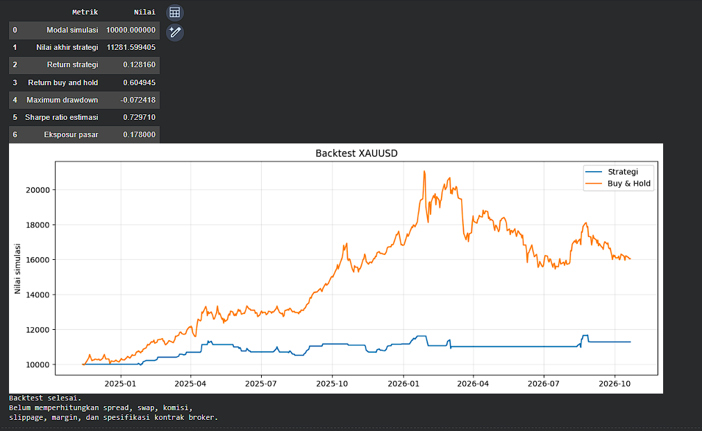
The strategy equity curve is calculated by compounding the simulated returns from an initial capital of 10,000 units. A buy-and-hold equity curve is calculated using the same initial capital for comparison.

The evaluation includes the final simulated equity, total strategy return, buy-and-hold return, maximum drawdown, estimated Sharpe ratio, and market exposure.

Maximum drawdown measures the largest percentage decline from a historical equity peak. The estimated Sharpe ratio compares the average periodic strategy return with its standard deviation and annualizes the result using a factor of 252. This annualization assumes daily trading observations and should be interpreted cautiously if the dataset contains a different frequency.

The final chart compares the strategy equity curve with the buy-and-hold benchmark. The simulation does not account for spreads, commissions, swap charges, slippage, margin requirements, or broker-specific contract specifications. It also does not implement short positions or the configured risk-reward parameter. Therefore, the results represent a simplified historical simulation rather than a complete execution model.

Code — Cell 5

# Position based on the previous candle's signal
data["Position"] = (
    data["Signal"] == "POTENTIAL BUY"
).astype(float).shift(1).fillna(0)


# Strategy returns
data["StrategyReturn"] = (
    data["Position"]
    * data["Return"].fillna(0)
)


# Strategy equity
data["StrategyEquity"] = (
    INITIAL_CAPITAL
    * (1 + data["StrategyReturn"]).cumprod()
)


# Buy-and-hold benchmark
data["BuyHoldEquity"] = (
    INITIAL_CAPITAL
    * (1 + data["Return"].fillna(0)).cumprod()
)


def max_drawdown(equity):
    return (
        equity / equity.cummax() - 1
    ).min()


# Estimated Sharpe ratio
daily_std = data["StrategyReturn"].std()

sharpe = (
    data["StrategyReturn"].mean()
    / daily_std
    * np.sqrt(252)
    if pd.notna(daily_std) and daily_std > 0
    else np.nan
)


# Performance metrics
metrics = pd.DataFrame({
    "Metric": [
        "Initial Capital",
        "Final Strategy Equity",
        "Strategy Total Return",
        "Buy-and-Hold Return",
        "Maximum Drawdown",
        "Estimated Sharpe Ratio",
        "Market Exposure"
    ],
    "Value": [
        INITIAL_CAPITAL,
        data["StrategyEquity"].iloc[-1],
        (
            data["StrategyEquity"].iloc[-1]
            / INITIAL_CAPITAL - 1
        ),
        (
            data["BuyHoldEquity"].iloc[-1]
            / INITIAL_CAPITAL - 1
        ),
        max_drawdown(data["StrategyEquity"]),
        sharpe,
        data["Position"].mean()
    ]
})


display(metrics)


# Equity curve comparison
plt.figure(figsize=(14, 5))

plt.plot(
    data.index,
    data["StrategyEquity"],
    label="Strategy"
)

plt.plot(
    data.index,
    data["BuyHoldEquity"],
    label="Buy and Hold"
)

plt.title("XAUUSD Backtesting Results")
plt.ylabel("Simulated Equity")
plt.legend()
plt.grid(alpha=0.3)
plt.tight_layout()
plt.show()


print("Backtesting completed.")
print(
    "The simulation excludes spread, swap, commissions, "
    "slippage, margin, and broker contract specifications."
)

3. Results and Discussion

3.1. Historical Price Data and Technical Indicators

The framework produces a structured historical dataset containing OHLC prices and the calculated technical indicators. The final observations can be displayed in tabular form, allowing the analyst to examine the most recent price movements and their relationship with the selected indicators.

SMA20 and SMA50 provide a basic representation of the relative trend direction. MACD and its signal line provide additional momentum information, while RSI14 measures the relationship between recent upward and downward price movements. Bollinger Bands complement these indicators by illustrating the recent variability of closing prices.

The interpretation of these indicators should consider their combined behavior. For example, a bullish moving-average configuration may indicate an upward trend, but it does not guarantee continued appreciation. Momentum changes, volatility, and nearby historical price boundaries may influence the quality of a potential trading setup.

The actual market interpretation must be based on the values produced by executing the program. Because the source code has not been accompanied by verified execution results, this article does not report specific current prices or numerical indicator readings.

3.2. Potential Trading Signals

The signal-generation component classifies market observations into potential buy, potential sell, or wait/mixed conditions.

A potential buy signal indicates that the predefined trend, momentum, and RSI requirements are satisfied simultaneously. A potential sell signal indicates that the corresponding bearish requirements are met. A wait/mixed signal indicates that the conditions are not sufficiently aligned according to the selected rules.

This classification provides a consistent method for screening historical price observations. However, the number of generated signals and their subsequent profitability must be evaluated using actual market data.

The thresholds used in this framework are predefined strategy parameters. They should not be interpreted as universally optimal settings, and additional research is necessary to determine whether alternative parameters produce more robust results.

3.3. Backtesting Performance

The backtesting stage calculates the simulated equity of the rule-based strategy and compares it with a buy-and-hold benchmark. The resulting metrics provide several perspectives on historical performance.

Total strategy return measures the percentage change between the initial capital and the final simulated equity. Maximum drawdown estimates the largest decline from a previous equity peak. The estimated Sharpe ratio summarizes the relationship between average returns and return variability, while market exposure indicates the proportion of observations during which the strategy holds a position.

These metrics must be interpreted together. A strategy with a positive return may still experience substantial drawdowns, while a higher Sharpe ratio does not independently establish that a strategy will remain profitable under different market conditions.

The backtest is intentionally simplified. It only models long exposure and does not execute short positions when bearish signals appear. It also assumes that the strategy can obtain the returns implied by consecutive closing prices without incorporating trading costs or detailed order execution. Consequently, actual trading performance may differ substantially from the simulated results.

Further evaluation should include out-of-sample testing, walk-forward validation, sensitivity analysis, and realistic transaction costs. Additional work should also address position sizing, stop-loss execution, take-profit rules, and the effects of leverage before the strategy is considered for practical deployment.

3.4. Limitations and Practical Implications

The framework demonstrates how an API-based data pipeline can be combined with technical indicators, visualization, and historical strategy evaluation. Its modular structure allows the analyst to inspect individual stages and modify the indicator parameters or trading conditions as required.

Nevertheless, several limitations remain. The analysis depends on the quality and completeness of the API data, the correct identification of candlestick fields, and the assumptions used in the backtesting procedure. In addition, the strategy rules have not been statistically validated, and the program does not incorporate macroeconomic variables or fundamental gold-market information.

The results should therefore be used as preliminary analytical support rather than as an automated recommendation to enter or exit a position. More comprehensive testing is necessary to establish whether the strategy offers a reliable advantage over a suitable benchmark.

4. Conclusion

This article presents a Python-based framework for analyzing XAUUSD using the MarketFlow All-in-One Market Finance API. The implementation integrates historical market data retrieval, OHLC data processing, SMA20 and SMA50, RSI14, MACD, Bollinger Bands, rolling support and resistance, rule-based trading signals, and historical backtesting.

The framework provides a reproducible workflow for examining gold price behavior and evaluating predefined technical trading rules. Its visualizations and performance metrics can help organize market observations and identify areas that require further investigation.

However, the framework does not establish that the proposed strategy is profitable. Its performance must be assessed using actual API responses, realistic execution assumptions, transaction costs, and independent validation data. Future improvements should include two-sided position management, risk-based position sizing, stop-loss and take-profit implementation, and out-of-sample evaluation.

Overall, the proposed system offers a foundation for developing more comprehensive quantitative trading research. Its practical value will depend on the quality of the market data, the robustness of the trading rules, and the rigor of subsequent performance evaluation.

Result:

SEO Metadata

SEO Title

Python XAUUSD Trading Analysis and Backtesting Using MarketFlow API

SEO Description

Learn how to analyze XAUUSD using Python and MarketFlow API. Explore SMA, RSI, MACD, Bollinger Bands, trading signals, price visualization, and backtesting.

SEO Keywords

XAUUSD analysis, Python trading analysis, gold trading strategy, MarketFlow API, XAUUSD backtesting, technical analysis Python, SMA indicator, RSI 14, MACD trading, Bollinger Bands, algorithmic trading, gold price analysis, trading strategy evaluation.