
Financial market analysis requires a combination of price-based indicators and information about institutional investment activity. Traders who focus exclusively on price movements may overlook broader market conditions, while those who examine institutional transactions without considering technical trends may have difficulty identifying suitable market entry opportunities. Integrating both approaches can provide a more comprehensive framework for evaluating financial markets.
Gold, traded under the XAUUSD symbol, is one of the most actively monitored instruments in global financial markets. Its price is influenced by several factors, including US dollar movements, interest rate expectations, inflation, geopolitical developments, and investor demand for safe-haven assets. Because of these influences, XAUUSD can experience substantial price fluctuations, making systematic market analysis important for identifying potential trading opportunities.
Technical analysis provides several tools for examining these movements. Moving averages help identify the prevailing market trend, the Relative Strength Index (RSI) evaluates momentum, the Moving Average Convergence Divergence (MACD) identifies changes in momentum, and the Average True Range (ATR) measures price volatility. Support and resistance levels provide additional information about recent price boundaries.
In addition to technical indicators, institutional flow analysis can provide another perspective on financial market activity. Institutional disclosures and transaction records can reveal information about reported investment positions, asset allocations, and investment activities. Examining these records can help analysts understand the behavior of selected institutional investors, although historical disclosures do not necessarily represent their current positions.
Python provides a flexible environment for combining these analytical approaches. Through financial APIs, historical price data and institutional flow records can be retrieved, processed, normalized, and transformed into structured analytical datasets. Libraries such as Requests, Pandas, NumPy, and Matplotlib support automated data collection, statistical calculations, and financial visualization.
This article presents MarketFlow Trader Analyzer, a Python-based financial analysis framework that integrates XAUUSD technical analysis with institutional flow monitoring through the MarketFlow All-in-One Market Finance API. The system uses OANDA:XAUUSD as its primary instrument and retrieves historical daily price data with a configured range of 100 observations.
The institutional analysis focuses on Warren Buffett using the investor identifier warren-buffett, with a reporting period from January 1, 2023, to December 31, 2024. The framework processes the returned institutional records and automatically identifies available date, asset, transaction, and value-related columns.
The technical analysis component calculates SMA 20, SMA 50, EMA 20, EMA 50, RSI 14, MACD, MACD Signal, MACD Histogram, ATR 14, daily returns, and rolling 20-period support and resistance levels.
These indicators are then integrated into a trader intelligence dashboard that evaluates market trend, momentum, RSI conditions, and technical scoring. The final system generates a BULLISH, BEARISH, or NEUTRAL / WAIT market classification and presents a corresponding trading scenario.
The objective is to demonstrate how Python can combine historical gold price analysis and institutional flow information within a reproducible financial research workflow. The resulting dashboard is intended to support market observation and trading research rather than provide guaranteed price predictions or automatic investment recommendations.
2. Methodology
MarketFlow Trader Analyzer is organized into five computational cells.
Cell 1 — Configuration and Libraries: imports the required Python libraries, configures RapidAPI authentication, establishes OANDA:XAUUSD as the primary instrument, and defines the technical and institutional analysis parameters.
Cell 2 — API Data Collection: retrieves historical XAUUSD price data and institutional flow records associated with Warren Buffett.
Cell 3 — Technical Analysis Engine: normalizes historical OHLC data, resolves duplicate columns, processes timestamps, and calculates technical indicators, daily returns, support, and resistance.
Cell 4 — Institutional Flow Analysis: normalizes institutional records, automatically detects important data columns, examines reporting dates, and summarizes transaction activity.
Cell 5 — Trader Intelligence Dashboard: evaluates trend, momentum, RSI conditions, technical scores, market bias, trading scenarios, visualizations, and CSV exports.
2.1. Historical XAUUSD Data Acquisition
The system retrieves historical gold price information through the MarketFlow endpoint:
/v2/chart/price
The request uses the following configuration:
Parameter | Value |
|---|---|
Instrument | OANDA:XAUUSD |
Historical range | 100 |
Timeframe | Daily (D) |
Timezone | Asia/Jakarta |
The API response is processed into a structured OHLC dataset containing opening, highest, lowest, and closing prices. When available, timestamps are converted into the Asia/Jakarta timezone.
2.2. Moving Average Analysis
The framework calculates two types of moving averages: Simple Moving Average (SMA) and Exponential Moving Average (EMA).
SMA 20 and SMA 50 calculate average closing prices over 20 and 50 observations, respectively.
EMA 20 and EMA 50 apply greater weight to more recent price observations.
The dashboard uses EMA 20 and EMA 50 to determine the trend classification:
Bullish: EMA 20 is above EMA 50.
Bearish: EMA 20 is below EMA 50.
2.3. Relative Strength Index
RSI 14 evaluates the magnitude of recent upward and downward price movements.
The system uses the following classification:
RSI value | Condition |
|---|---|
70 or above | Overbought |
30 or below | Oversold |
Between 30 and 70 | Neutral |
For technical scoring, RSI values between 50 and 70 contribute one bullish point, while values between 30 and 50 contribute one bearish point.
2.4. MACD Momentum Analysis
The Moving Average Convergence Divergence indicator is calculated using the difference between EMA 12 and EMA 26.
A 9-period EMA of the MACD line is used as the signal line.
The dashboard determines momentum through the following comparison:
Bullish momentum: MACD is above MACD Signal.
Bearish momentum: MACD is below MACD Signal.
The MACD Histogram is calculated as the difference between the MACD line and its signal line and is used in the visualization.
2.5. Average True Range
ATR 14 measures price volatility using the True Range of each observation.
The True Range is determined from three components:
\[ TR=\max \begin{cases} High-Low\\ |High-PreviousClose|\\ |Low-PreviousClose| \end{cases} \]
The system calculates ATR using a 14-period rolling average of the True Range.
2.6. Support and Resistance
The framework calculates support and resistance using rolling 20-period price boundaries.
\[ Support_{20}=\min(Low_{20}) \]
\[ Resistance_{20}=\max(High_{20}) \]
These levels represent the lowest low and highest high within the latest 20 observations.
2.7. Institutional Flow Analysis
The institutional flow component retrieves records through the endpoint:
/smartmoney/institutional-flow
The selected institution is Warren Buffett, identified by warren-buffett, with a reporting period from January 1, 2023, to December 31, 2024.
The system automatically detects available columns based on keywords associated with:
Dates and reporting periods.
Asset names and ticker symbols.
Transaction actions and types.
Values, shares, quantities, holdings, and portfolio weights.
The purpose of this process is to make the analysis adaptable to the available API response structure without assuming that every response uses identical column names.
2.8. Technical Scoring and Market Bias
The final dashboard combines three analytical components:
Component | Bullish condition | Bearish condition |
|---|---|---|
Trend | EMA 20 above EMA 50 | EMA 20 below EMA 50 |
Momentum | MACD above Signal | MACD below Signal |
RSI | 50–70 | 30–50 |
Each satisfied condition contributes one point in its corresponding direction.
The final market bias is determined as follows:
Score of 2 or higher: BULLISH.
Score of -2 or lower: BEARISH.
Other scores: NEUTRAL / WAIT.
The maximum theoretical score is +3 and the minimum is -3. RSI values outside the scoring ranges do not contribute an additional point.
3. Implementation and Python Code
The following implementation follows the uploaded marketflow_trader_analyzer.py file. The complete program is divided into five cells to make execution and troubleshooting easier in Google Colab.
Cell 1 — Configuration and Libraries
The first cell imports the required libraries and establishes the API connection through RapidAPI. It also defines the primary trading instrument, historical data range, timeframe, timezone, selected institution, and technical indicator periods.
The API key is entered using getpass so that the credential is not displayed directly in the notebook output.
Code — Cell 1
# ==========================================
# CELL 1: CONFIGURATION & LIBRARIES
# ==========================================

import requests
import json
import warnings
import getpass
import numpy as np
import pandas as pd
import matplotlib.pyplot as plt

from datetime import datetime

warnings.filterwarnings("ignore")

pd.set_option("display.max_columns", 50)
pd.set_option("display.width", 180)

# API CONFIGURATION
BASE_URL = "https://marketflow-all-in-one-market-finance-api.p.rapidapi.com"

API_HOST = "marketflow-all-in-one-market-finance-api.p.rapidapi.com"

API_KEY = getpass.getpass("Masukkan RapidAPI Key: ")

HEADERS = {
    "x-rapidapi-host": API_HOST,
    "x-rapidapi-key": API_KEY
}

# GOLD CONFIGURATION
SYMBOL = "OANDA:XAUUSD"
PRICE_RANGE = 100
TIMEFRAME = "D"
TIMEZONE = "Asia/Jakarta"

# INSTITUTIONAL FLOW CONFIGURATION
INSTITUTION = "warren-buffett"

START_DATE = "2023-01-01"
END_DATE = "2024-12-31"

# ANALYSIS CONFIGURATION
RSI_PERIOD = 14
ATR_PERIOD = 14

print("=" * 60)
print("MARKETFLOW TRADER ANALYZER")
print("=" * 60)

print("Instrument :", SYMBOL)
print("Timeframe  :", TIMEFRAME)
print("Range      :", PRICE_RANGE)
print("Institution:", INSTITUTION)
print("Status     : Configuration Ready")
Cell 2 — API Data Collection
The second cell defines the marketflow_request() function to communicate with the MarketFlow API.
The function sends authenticated GET requests, applies a 30-second timeout, checks the HTTP response status, and returns the decoded JSON response.
Two datasets are retrieved:
Historical XAUUSD daily price information through
/v2/chart/price.Institutional flow records through
/smartmoney/institutional-flow.
The responses are displayed in JSON format to allow inspection of their structure before data processing.
Code — Cell 2
# ==========================================
# CELL 2: API DATA COLLECTION
# ==========================================

def marketflow_request(endpoint, params):

    url = f"{BASE_URL}{endpoint}"

    response = requests.get(
        url,
        headers=HEADERS,
        params=params,
        timeout=30
    )

    print(f"API: {endpoint}")
    print("HTTP Status:", response.status_code)

    response.raise_for_status()

    return response.json()


# ==========================================
# 1. XAUUSD PRICE DATA
# ==========================================

price_raw = marketflow_request(
    "/v2/chart/price",
    {
        "range": PRICE_RANGE,
        "timeframe": TIMEFRAME,
        "timezone": TIMEZONE,
        "symbol": SYMBOL
    }
)


# ==========================================
# 2. INSTITUTIONAL FLOW
# ==========================================

institutional_raw = marketflow_request(
    "/smartmoney/institutional-flow",
    {
        "start_date": START_DATE,
        "slug": INSTITUTION,
        "end_date": END_DATE
    }
)


# ==========================================
# DISPLAY API RESPONSE
# ==========================================

print("\nPRICE DATA STRUCTURE")

print(json.dumps(
    price_raw,
    indent=2
)[:2500])


print("\nINSTITUTIONAL FLOW STRUCTURE")

print(json.dumps(
    institutional_raw,
    indent=2
)[:2500])


print("\nDATA COLLECTION COMPLETED")
Cell 3 — Technical Analysis Engine
The third cell transforms the raw XAUUSD API response into a structured OHLC DataFrame.
The extract_records() function recursively searches the JSON response for lists of records and selects the longest available list. This helps accommodate nested API response structures.
The system then standardizes column names, maps common OHLC aliases, and resolves duplicate columns by retaining the first available non-null value.
After validating the required OHLC fields, timestamps are converted into the configured timezone. The program also removes invalid observations and duplicate timestamps.
The technical analysis engine calculates SMA, EMA, RSI, MACD, ATR, daily returns, and rolling support and resistance.
Code — Cell 3
# ==========================================
# CELL 3: TECHNICAL ANALYSIS ENGINE
# FIXED VERSION
# ==========================================

def extract_records(data):

    candidates = []

    def search(obj):

        if isinstance(obj, list):

            if obj and all(isinstance(x, dict) for x in obj):
                candidates.append(obj)

            else:
                for item in obj:
                    search(item)

        elif isinstance(obj, dict):

            for value in obj.values():
                search(value)

    search(data)

    if not candidates:
        raise ValueError("Data OHLC tidak ditemukan.")

    return max(candidates, key=len)


# ==========================================
# NORMALIZE PRICE DATA
# ==========================================

price_df = pd.DataFrame(
    extract_records(price_raw)
)

price_df.columns = [
    str(c).lower().strip()
    for c in price_df.columns
]

# Mapping kolom API
column_mapping = {
    "t": "time",
    "timestamp": "time",
    "datetime": "time",
    "date": "time",
    "o": "open",
    "h": "high",
    "l": "low",
    "c": "close",
    "v": "volume",
    "vol": "volume",
    "price": "close"
}

price_df.rename(
    columns=column_mapping,
    inplace=True
)


# ==========================================
# FIX DUPLICATE COLUMNS
# ==========================================

# Gabungkan kolom dengan nama sama.
# Nilai pertama yang tidak kosong akan dipertahankan.

if price_df.columns.duplicated().any():

    print("Duplicate columns detected.")

    price_df = (
        price_df.T
        .groupby(level=0, sort=False)
        .first()
        .T
    )

    print("Duplicate columns fixed.")


print("\nAVAILABLE COLUMNS:")
print(price_df.columns.tolist())


# ==========================================
# VALIDATE OHLC
# ==========================================

required = [
    "open",
    "high",
    "low",
    "close"
]

missing = [
    col for col in required
    if col not in price_df.columns
]

if missing:

    raise ValueError(
        f"Missing OHLC columns: {missing}. "
        f"Available: {price_df.columns.tolist()}"
    )


# ==========================================
# TIMESTAMP PROCESSING
# ==========================================

if "time" in price_df.columns:

    time_series = price_df["time"]

    # Pastikan time berbentuk Series
    if isinstance(time_series, pd.DataFrame):
        time_series = time_series.iloc[:, 0]

    numeric_time = pd.to_numeric(
        time_series,
        errors="coerce"
    )

    if numeric_time.notna().mean() > 0.8:

        median_time = numeric_time.dropna().median()

        unit = (
            "ms" if median_time > 1e11
            else "s"
        )

        price_df["time"] = pd.to_datetime(
            numeric_time,
            unit=unit,
            utc=True
        ).dt.tz_convert(TIMEZONE)

    else:

        price_df["time"] = pd.to_datetime(
            time_series,
            errors="coerce",
            utc=True
        ).dt.tz_convert(TIMEZONE)

    price_df = price_df.dropna(
        subset=["time"]
    )

    price_df = price_df.sort_values(
        "time"
    )

    price_df = price_df.set_index(
        "time"
    )


# ==========================================
# CONVERT NUMERIC OHLC
# ==========================================

for col in required:

    price_df[col] = pd.to_numeric(
        price_df[col],
        errors="coerce"
    )

price_df.dropna(
    subset=required,
    inplace=True
)

price_df = price_df[
    ~price_df.index.duplicated(keep="last")
]


# ==========================================
# MOVING AVERAGES
# ==========================================

price_df["SMA20"] = (
    price_df["close"].rolling(20).mean()
)

price_df["SMA50"] = (
    price_df["close"].rolling(50).mean()
)

price_df["EMA20"] = (
    price_df["close"].ewm(
        span=20,
        adjust=False
    ).mean()
)

price_df["EMA50"] = (
    price_df["close"].ewm(
        span=50,
        adjust=False
    ).mean()
)


# ==========================================
# RSI 14
# ==========================================

delta = price_df["close"].diff()

gain = delta.clip(lower=0)

loss = -delta.clip(upper=0)

avg_gain = gain.rolling(14).mean()

avg_loss = loss.rolling(14).mean()

rs = avg_gain / avg_loss.replace(0, np.nan)

price_df["RSI"] = (
    100 - (100 / (1 + rs))
)

price_df.loc[
    (avg_loss == 0) & (avg_gain > 0),
    "RSI"
] = 100

price_df.loc[
    (avg_gain == 0) & (avg_loss > 0),
    "RSI"
] = 0

price_df.loc[
    (avg_gain == 0) & (avg_loss == 0),
    "RSI"
] = 50


# ==========================================
# MACD
# ==========================================

ema12 = price_df["close"].ewm(
    span=12,
    adjust=False
).mean()

ema26 = price_df["close"].ewm(
    span=26,
    adjust=False
).mean()

price_df["MACD"] = ema12 - ema26

price_df["MACD_SIGNAL"] = (
    price_df["MACD"].ewm(
        span=9,
        adjust=False
    ).mean()
)

price_df["MACD_HIST"] = (
    price_df["MACD"] -
    price_df["MACD_SIGNAL"]
)


# ==========================================
# ATR 14
# ==========================================

previous_close = price_df["close"].shift(1)

tr = pd.concat(
    [
        price_df["high"] - price_df["low"],

        (price_df["high"] - previous_close).abs(),

        (price_df["low"] - previous_close).abs()

    ],
    axis=1
).max(axis=1)

price_df["ATR"] = tr.rolling(14).mean()


# ==========================================
# DAILY RETURN
# ==========================================

price_df["RETURN"] = (
    price_df["close"].pct_change() * 100
)


# ==========================================
# SUPPORT & RESISTANCE
# ==========================================

price_df["SUPPORT_20"] = (
    price_df["low"].rolling(20).min()
)

price_df["RESISTANCE_20"] = (
    price_df["high"].rolling(20).max()
)


# ==========================================
# FINAL VALIDATION
# ==========================================

print("\n" + "=" * 60)

print("TECHNICAL ANALYSIS COMPLETED")

print("=" * 60)

print("Total Candles :", len(price_df))

print("Latest Close  :", price_df["close"].iloc[-1])

print("Latest RSI    :", price_df["RSI"].iloc[-1])

print("Latest ATR    :", price_df["ATR"].iloc[-1])

print("\nFINAL DATA:")

display(
    price_df.tail(15).round(3)
)
Cell 4 — Institutional Flow Analysis
The fourth cell processes the institutional flow response and converts the available records into a normalized DataFrame.
The system reuses the extract_records() function from Cell 3 to locate the institutional records within the API response.
It then automatically detects important columns using keyword matching. The detected fields are grouped into date, asset, transaction action, and value categories.
If a date column is available, the program converts it into a datetime format and displays the earliest and latest reporting dates. If transaction action information is available, the program calculates the frequency of each reported action.
Finally, the first 30 institutional records are displayed for inspection.
This approach allows the analyst to explore the structure and distribution of institutional flow data without assuming that all API responses contain identical field names.
Code — Cell 4
# ==========================================
# CELL 4: INSTITUTIONAL FLOW ANALYSIS
# ==========================================

institutional_df = pd.json_normalize(
    extract_records(institutional_raw),
    sep="_"
)

institutional_df.columns = [
    str(c).lower().strip()
    for c in institutional_df.columns
]


# ==========================================
# DETECT IMPORTANT COLUMNS
# ==========================================

def detect_columns(columns, keywords):

    return [
        col for col in columns
        if any(
            keyword in col
            for keyword in keywords
        )
    ]


date_columns = detect_columns(
    institutional_df.columns,
    ["date", "time", "reported", "filing"]
)

asset_columns = detect_columns(
    institutional_df.columns,
    ["ticker", "symbol", "company", "name"]
)

action_columns = detect_columns(
    institutional_df.columns,
    ["action", "transaction", "side", "type"]
)

value_columns = detect_columns(
    institutional_df.columns,
    ["value", "shares", "quantity", "holding", "weight"]
)


# ==========================================
# DISPLAY AVAILABLE DATA
# ==========================================

print("=" * 60)
print("INSTITUTIONAL FLOW ANALYSIS")
print("=" * 60)

print("Institution:", INSTITUTION)

print("\nDetected Date Columns:")
print(date_columns)

print("\nDetected Asset Columns:")
print(asset_columns)

print("\nDetected Action Columns:")
print(action_columns)

print("\nDetected Value Columns:")
print(value_columns)


# ==========================================
# DATA PREPARATION
# ==========================================

if date_columns:

    institutional_df[date_columns[0]] = pd.to_datetime(
        institutional_df[date_columns[0]],
        errors="coerce"
    )

    print("\nDate Range:")

    print(
        institutional_df[date_columns[0]].min(),
        "to",
        institutional_df[date_columns[0]].max()
    )


# ==========================================
# ACTION DISTRIBUTION
# ==========================================

if action_columns:

    action_col = action_columns[0]

    print("\nInstitutional Activity Distribution")

    display(
        institutional_df[action_col]
        .astype(str)
        .str.lower()
        .value_counts()
        .to_frame("Total Records")
    )


# ==========================================
# INSTITUTIONAL DATA TABLE
# ==========================================

print("\nINSTITUTIONAL TRANSACTIONS")

display(
    institutional_df.head(30)
)

print("\nInstitutional analysis completed.")
Cell 5 — Trader Intelligence Dashboard
The fifth cell integrates the technical analysis results into the final MarketFlow Trader Intelligence dashboard.
The latest and previous closing prices are used to calculate the daily percentage change. The system then evaluates the EMA trend, MACD momentum, and RSI condition.
The technical scoring model assigns positive or negative points according to the three indicators. Based on the resulting score, the system generates a BULLISH, BEARISH, or NEUTRAL / WAIT market classification.
The dashboard also displays the latest support, resistance, ATR, and technical indicator values.
Three visualization panels are generated:
XAUUSD price action with EMA 20, EMA 50, support, and resistance.
RSI momentum with 30, 50, and 70 reference levels.
MACD analysis with the MACD line, signal line, and histogram.
Finally, the processed price data and institutional flow records are exported into separate CSV files.
Code — Cell 5
# ==========================================
# CELL 5: TRADER INTELLIGENCE DASHBOARD
# ==========================================

latest = price_df.iloc[-1]

previous = price_df.iloc[-2]

close = float(latest["close"])

change = (
    (close / previous["close"]) - 1
) * 100


# ==========================================
# TREND ANALYSIS
# ==========================================

if latest["EMA20"] > latest["EMA50"]:

    trend = "BULLISH"

else:

    trend = "BEARISH"


# ==========================================
# MOMENTUM ANALYSIS
# ==========================================

if latest["MACD"] > latest["MACD_SIGNAL"]:

    momentum = "BULLISH"

else:

    momentum = "BEARISH"


# ==========================================
# RSI ANALYSIS
# ==========================================

rsi = latest["RSI"]

if pd.isna(rsi):

    rsi_condition = "INSUFFICIENT DATA"

elif rsi >= 70:

    rsi_condition = "OVERBOUGHT"

elif rsi <= 30:

    rsi_condition = "OVERSOLD"

else:

    rsi_condition = "NEUTRAL"


# ==========================================
# SUPPORT & RESISTANCE
# ==========================================

support = price_df["low"].tail(20).min()

resistance = price_df["high"].tail(20).max()

atr = latest["ATR"]


# ==========================================
# MARKET SCORING
# ==========================================

score = 0

# Trend
score += (
    1 if trend == "BULLISH" else -1
)

# Momentum
score += (
    1 if momentum == "BULLISH" else -1
)

# RSI
if pd.notna(rsi):

    if 50 < rsi < 70:
        score += 1

    elif 30 < rsi < 50:
        score -= 1


# ==========================================
# MARKET BIAS
# ==========================================

if score >= 2:

    market_bias = "BULLISH"

elif score <= -2:

    market_bias = "BEARISH"

else:

    market_bias = "NEUTRAL / WAIT"


# ==========================================
# DASHBOARD OUTPUT
# ==========================================

print("\n")
print("=" * 65)
print("              MARKETFLOW TRADER INTELLIGENCE")
print("=" * 65)

print(f"Instrument       : {SYMBOL}")

print(f"Last Price       : {close:,.3f}")

print(f"Daily Change     : {change:+.2f}%")

print("-" * 65)

print(f"Trend            : {trend}")

print(f"Momentum         : {momentum}")

print(f"RSI              : {rsi:.2f}" if pd.notna(rsi) else "RSI              : N/A")

print(f"RSI Condition    : {rsi_condition}")

print(f"ATR              : {atr:,.3f}" if pd.notna(atr) else "ATR              : N/A")

print("-" * 65)

print(f"Support          : {support:,.3f}")

print(f"Resistance       : {resistance:,.3f}")

print("-" * 65)

print(f"Technical Score  : {score}/3")

print(f"MARKET BIAS      : {market_bias}")

print("=" * 65)


# ==========================================
# TRADING SCENARIO
# ==========================================

print("\nTRADING SCENARIO")

if market_bias == "BULLISH":

    print("Potential Setup: BUY")

    print("1. Wait for bullish pullback.")

    print("2. Observe EMA20 and support.")

    print("3. Wait for bullish candle confirmation.")

elif market_bias == "BEARISH":

    print("Potential Setup: SELL")

    print("1. Wait for bearish pullback.")

    print("2. Observe EMA20 and resistance.")

    print("3. Wait for bearish candle confirmation.")

else:

    print("Potential Setup: WAIT")

    print("1. Wait for market structure confirmation.")

    print("2. Monitor breakout and retest.")

    print("3. Avoid entering during unclear momentum.")


# ==========================================
# CHART VISUALIZATION
# ==========================================

fig, axes = plt.subplots(
    3,
    1,
    figsize=(16, 12),
    sharex=True,
    gridspec_kw={
        "height_ratios": [3, 1, 1]
    }
)

x = price_df.index

# PRICE CHART

axes[0].plot(
    x,
    price_df["close"],
    label="XAUUSD Close",
    linewidth=1.5
)

axes[0].plot(
    x,
    price_df["EMA20"],
    label="EMA 20"
)

axes[0].plot(
    x,
    price_df["EMA50"],
    label="EMA 50"
)

axes[0].axhline(
    support,
    linestyle="--",
    label="Support"
)

axes[0].axhline(
    resistance,
    linestyle="--",
    label="Resistance"
)

axes[0].set_title(
    "XAUUSD PRICE ACTION"
)

axes[0].legend()

axes[0].grid(alpha=0.2)


# RSI CHART

axes[1].plot(
    x,
    price_df["RSI"],
    label="RSI 14"
)

axes[1].axhline(70, linestyle="--")

axes[1].axhline(30, linestyle="--")

axes[1].axhline(50, linestyle=":")

axes[1].set_ylim(0, 100)

axes[1].set_title("RSI MOMENTUM")

axes[1].legend()

axes[1].grid(alpha=0.2)


# MACD CHART

axes[2].bar(
    x,
    price_df["MACD_HIST"],
    label="MACD Histogram"
)

axes[2].plot(
    x,
    price_df["MACD"],
    label="MACD"
)

axes[2].plot(
    x,
    price_df["MACD_SIGNAL"],
    label="Signal"
)

axes[2].set_title("MACD ANALYSIS")

axes[2].legend()

axes[2].grid(alpha=0.2)


plt.tight_layout()

plt.show()


# ==========================================
# EXPORT ANALYSIS
# ==========================================

price_df.to_csv(
    "marketflow_xauusd_analysis.csv"
)

institutional_df.to_csv(
    "marketflow_institutional_flow.csv",
    index=False
)

print("\nEXPORT COMPLETED")

print("1. marketflow_xauusd_analysis.csv")

print("2. marketflow_institutional_flow.csv")


print("\nDISCLAIMER")

print(
    "Analisis ini merupakan alat bantu keputusan trading, "
    "bukan jaminan profit atau rekomendasi investasi."
)
Result:
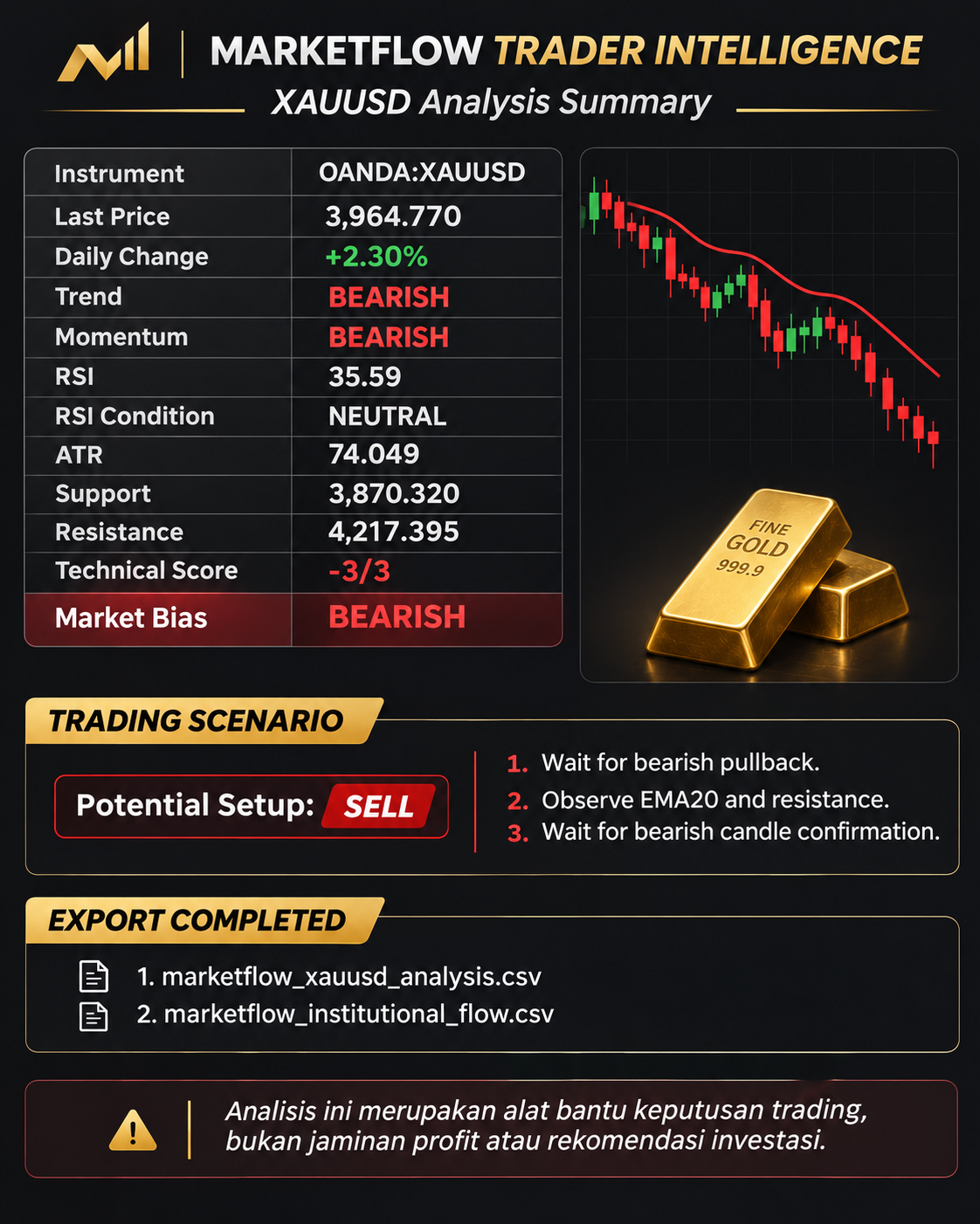
4. Results and Discussion
4.1. XAUUSD Historical Price Analysis
The historical price analysis module retrieves daily XAUUSD observations and converts them into a structured dataset containing OHLC information.
The framework requests 100 historical observations using the MarketFlow API and processes the available records into a time-indexed DataFrame.
The resulting dataset provides the foundation for calculating moving averages, momentum indicators, volatility measurements, and recent price boundaries.
The latest closing price is subsequently compared with the previous observation to calculate the percentage change:
\[ Daily\ Change = \left( \frac{Close_t}{Close_{t-1}}-1 \right)\times100 \]
Because the system uses daily timeframe data, this calculation represents the change between consecutive available observations.
4.2. Technical Trend and Momentum Evaluation
The technical analysis engine combines moving averages and momentum indicators to evaluate the current market condition.
SMA 20 and SMA 50 provide additional information about the average closing price over different observation periods. EMA 20 and EMA 50 are used directly in the dashboard's trend classification.
When EMA 20 is above EMA 50, the system identifies a bullish trend. Conversely, when EMA 20 is below EMA 50, the system identifies a bearish trend.
Momentum is evaluated through the MACD and its signal line. A MACD value above the signal line represents bullish momentum, while a value below the signal line represents bearish momentum.
These two components provide separate assessments of market direction and momentum. Their combination helps identify whether the current trend and momentum measurements support the same directional interpretation.
4.3. RSI and Market Volatility
RSI 14 provides an additional perspective on price momentum.
Values of 70 or higher are classified as overbought, while values of 30 or lower are classified as oversold. Values between these thresholds are classified as neutral.
The dashboard also uses RSI in the technical scoring model. RSI between 50 and 70 contributes a bullish point, whereas RSI between 30 and 50 contributes a bearish point.
ATR 14 measures the average magnitude of recent price fluctuations through the rolling True Range calculation. A higher ATR indicates greater recent price movement, while a lower ATR indicates comparatively smaller fluctuations.
The combination of RSI and ATR provides information about momentum conditions and market volatility, complementing the trend and MACD measurements.
4.4. Support and Resistance Identification
The support and resistance module calculates the lowest low and highest high over the latest 20 observations.
These levels provide a reference for examining recent price boundaries.
Support represents the lowest observed price within the selected rolling period, while resistance represents the highest observed price.
The dashboard plots both levels alongside the closing price and EMA lines. This makes it easier to examine the relationship between recent price movements, trend direction, and the identified boundaries.
However, these calculations represent rolling historical extremes rather than independently validated reversal levels. They should therefore be interpreted as reference areas for further technical examination.
4.5. Institutional Flow Analysis
The institutional flow module retrieves records associated with Warren Buffett using the selected reporting period from 2023 to 2024.
The program automatically identifies available columns related to dates, assets, transaction actions, and financial values.
This functionality is useful when examining API datasets whose field names may differ from one response to another.
When date information is available, the system converts the selected date column into datetime format and displays the observed reporting period.
When transaction action information is available, the program calculates the frequency of the different reported actions. The first 30 records are also displayed to provide a closer examination of the returned institutional dataset.
The analysis is primarily descriptive. It identifies available institutional records and summarizes their structure and reported activity. It does not calculate institutional portfolio returns, determine the exact current holdings of the selected investor, or establish a direct causal relationship between institutional activity and XAUUSD price movements.
4.6. Technical Scoring and Market Bias
The Trader Intelligence Dashboard combines trend, momentum, and RSI conditions into a single technical score.
Each bullish or bearish confirmation contributes one point. The resulting score ranges from -3 to +3.
The system interprets the score using three market classifications:
Technical score | Market classification |
|---|---|
+2 to +3 | BULLISH |
-1 to +1 | NEUTRAL / WAIT |
-3 to -2 | BEARISH |
A bullish classification produces a potential BUY scenario, while a bearish classification produces a potential SELL scenario.
A neutral classification recommends waiting for clearer market structure and additional confirmation.
The dashboard also provides three suggested steps for each scenario, including monitoring pullbacks, observing EMA 20 and support or resistance, and waiting for candle confirmation.
These scenarios are conditional analytical outputs rather than automatic trade executions.
4.7. Technical Visualization and Data Export
The final dashboard generates three separate analytical panels.
Price Action Chart: displays the XAUUSD closing price, EMA 20, EMA 50, support, and resistance.
RSI Momentum Chart: presents RSI 14 with reference levels at 30, 50, and 70.
MACD Analysis Chart: displays the MACD line, signal line, and histogram to visualize momentum changes.
The system also exports two CSV files:
Output file | Description |
|---|---|
| Historical XAUUSD data and calculated technical indicators. |
| Normalized institutional flow records. |
These files can be used for further financial analysis, historical comparisons, and additional data-processing workflows.
4.8. Limitations and Future Improvements
Several limitations should be considered when interpreting the results.
First, the historical price dataset is limited to 100 observations. This provides a relatively short analytical window and may not capture different market regimes or longer-term price behavior.
Second, the technical indicators use specific calculation methods. RSI and ATR are calculated using simple rolling averages in the uploaded implementation rather than Wilder's smoothing method. Consequently, their values may differ from those displayed by other trading platforms.
Third, institutional flow analysis depends on the available API response. The program automatically selects the longest list of dictionary records and identifies columns using keyword matching. The selected list and detected fields should be inspected to ensure that they represent the intended institutional dataset.
Fourth, the institutional analysis is not integrated into the technical scoring formula. The final market bias is calculated exclusively from EMA trend, MACD momentum, and RSI conditions.
Fifth, the dashboard does not perform historical strategy backtesting. It generates a technical classification and potential trading scenario but does not calculate historical trading returns, transaction costs, position sizing, or maximum drawdown.
Future development could include expanding the historical dataset, incorporating additional institutional investors, comparing multiple reporting periods, integrating economic-calendar information, and implementing historical trading simulations.
Additional improvements could also include more advanced support and resistance detection, volatility-adjusted risk management, and automated monitoring of technical signal changes.
These developments would provide a more comprehensive foundation for combining institutional research and technical market analysis.
5. Conclusion
MarketFlow Trader Analyzer demonstrates how Python can integrate historical XAUUSD price analysis and institutional flow monitoring into a unified financial research framework.
The implementation combines MarketFlow API connectivity, OHLC data normalization, moving average calculations, RSI, MACD, ATR, daily returns, and rolling support and resistance measurements.
The institutional flow component complements the technical analysis by retrieving and organizing available investment records associated with Warren Buffett. Automatic column detection and reporting-date processing make it possible to inspect the returned institutional dataset systematically.
The final Trader Intelligence Dashboard combines EMA trend, MACD momentum, and RSI conditions to generate a technical score and classify the market as BULLISH, BEARISH, or NEUTRAL / WAIT. It also provides potential trading scenarios, visualizations, and downloadable CSV datasets.
Nevertheless, the system should be interpreted as an analytical decision-support framework rather than an automated prediction model. Its outputs depend on historical data quality, API response structure, indicator calculations, and the predefined technical scoring rules.
Future improvements should focus on expanding historical coverage, validating institutional records, integrating additional market information, and developing a comprehensive backtesting framework.
With these improvements, MarketFlow Trader Analyzer can serve as a foundation for systematic gold market research and the integration of technical analysis with institutional investment intelligence.