
Financial market analysis involves examining investment portfolios, asset allocation, and broader market performance to understand the characteristics of financial instruments and identify potential market conditions.
One important component of investment analysis is portfolio concentration. A portfolio with a substantial proportion of its reported value allocated to a limited number of holdings may have different exposure characteristics from a portfolio distributed across multiple assets. Consequently, evaluating portfolio allocation and concentration is an important part of financial intelligence.
Warren Buffett's investment portfolio provides an interesting subject for examining investment allocation and concentration. By retrieving reported portfolio information from financial data providers, analysts can identify individual holdings, examine their relative weights, and calculate concentration indicators.
In addition to portfolio analysis, global market performance provides another perspective for understanding financial market conditions. Market heatmaps are commonly used to visualize the relative performance of financial instruments and identify assets experiencing positive or negative movements.
Market breadth analysis extends this examination by evaluating the distribution of positive, negative, and neutral assets within a selected dataset. A market containing a greater number of positive-performing assets may indicate broader positive performance across the analyzed instruments, while a greater number of negative-performing assets may indicate weaker market breadth.
Python provides an effective environment for integrating portfolio and market performance information. Through libraries such as Requests, Pandas, NumPy, and Matplotlib, financial data can be retrieved from external APIs, transformed into structured datasets, evaluated quantitatively, and presented through visual dashboards.
This article presents the MarketFlow Trader Intelligence Analyzer, a Python-based financial analysis framework developed using the MarketFlow All-in-One Market Finance API through RapidAPI.
The system retrieves portfolio information through the /portofolio-checks endpoint using the investor identifier warren-buffett and reporting date June 30, 2024.
The framework also retrieves global heatmap information through the /global-heatmap endpoint using the symbol BTC.
The analytical workflow consists of five computational stages:
API configuration and authentication.
Portfolio and global heatmap data extraction.
JSON processing and data normalization.
Portfolio concentration and global market breadth analysis.
Dashboard visualization, Excel export, and report generation.
The portfolio analysis module identifies relevant asset information, portfolio values, allocation weights, and changes in reported holdings. It subsequently calculates Top 5 Concentration, Top 10 Concentration, and the Herfindahl-Hirschman Index.
Meanwhile, the global heatmap module examines the numerical performance field returned by the API and classifies assets into positive, negative, and neutral categories.
The primary objective of this project is to develop an automated financial intelligence workflow that combines portfolio concentration analysis with global market performance monitoring.
An important distinction is that the BTC parameter is used as the requested heatmap symbol. The actual instruments and performance metrics included in the returned response depend on the API's data structure. The resulting heatmap records should not automatically be interpreted as historical Bitcoin price candles or as a complete representation of the entire cryptocurrency market.
2. Methodology
The MarketFlow Trader Intelligence Analyzer is organized into five computational cells. Each cell performs a specific function within the financial data collection, processing, analysis, and visualization workflow.
Cell | Main function |
|---|---|
Cell 1 | Library imports, RapidAPI authentication, investor configuration, and output directory creation. |
Cell 2 | Warren Buffett portfolio and global heatmap data extraction. |
Cell 3 | JSON extraction, data cleaning, and normalization. |
Cell 4 | Portfolio allocation, concentration, HHI, and market breadth analysis. |
Cell 5 | Dashboard visualization, CSV exports, Excel workbook, and final report. |
2.1. System Configuration and API Authentication
The first computational cell establishes the analytical environment and API authentication.
The framework uses Requests for HTTP communication, Pandas for data processing, NumPy for numerical calculations, Matplotlib for visualization, JSON for handling API responses, and Pathlib for output directory management.
The API host is configured as:
marketflow-all-in-one-market-finance-api.p.rapidapi.com
Authentication is performed using a RapidAPI key entered through Python's getpass function. This prevents the key from being directly displayed in the notebook output.
The investor configuration uses warren-buffett as the portfolio identifier, with June 30, 2024, as the reporting date.
The global heatmap configuration uses BTC as its requested symbol.
All generated files are stored in the MARKETFLOW_TRADER_INTELLIGENCE directory.
Code — Cell 1: Configuration and Libraries
# ============================================================
# CELL 3: DATA PROCESSING & NORMALIZATION
# ============================================================

def extract_records(data):

    candidates = []

    def search(obj, path="root"):

        if isinstance(obj, list):

            records = [
                x for x in obj
                if isinstance(x, dict)
            ]

            if records:
                candidates.append((len(records), path, records))

            for i, value in enumerate(obj):
                search(value, f"{path}[{i}]")

        elif isinstance(obj, dict):

            for key, value in obj.items():
                search(value, f"{path}.{key}")

    search(data)

    if candidates:

        candidates.sort(
            key=lambda x: x[0],
            reverse=True
        )

        records = candidates[0][2]

        return pd.json_normalize(
            records,
            sep="_"
        )

    if isinstance(data, dict):

        return pd.json_normalize([data])

    return pd.DataFrame()


def clean_dataframe(df):

    if df.empty:
        return df

    df = df.copy()

    df.columns = [
        re.sub(
            r"[^a-zA-Z0-9_]+",
            "_",
            str(c)
        ).strip("_").lower()
        for c in df.columns
    ]

    for col in df.columns:

        if df[col].dtype == "object":

            converted = pd.to_numeric(
                df[col].astype(str)
                .str.replace(",", "", regex=False)
                .str.replace("%", "", regex=False),
                errors="coerce"
            )

            if converted.notna().sum() >= max(
                2,
                int(len(df) * 0.6)
            ):

                df[col] = converted

    return df


# EXTRACT DATA

portfolio_df = extract_records(
    portfolio_result["data"]
)

heatmap_df = extract_records(
    heatmap_result["data"]
)


# CLEAN DATA

portfolio_df = clean_dataframe(
    portfolio_df
)

heatmap_df = clean_dataframe(
    heatmap_df
)


print("=" * 60)
print("PORTFOLIO DATA")
print("=" * 60)

display(portfolio_df.head(10))


print("=" * 60)
print("GLOBAL HEATMAP DATA")
print("=" * 60)

display(heatmap_df.head(10))


print("\nDATA DIMENSIONS")

print("Portfolio:", portfolio_df.shape)
print("Heatmap:", heatmap_df.shape)
2.2. Financial Data Collection Through MarketFlow API
The second computational cell retrieves two financial datasets through the MarketFlow API.
The first dataset contains Warren Buffett's portfolio information. The system accesses the /portofolio-checks endpoint using the following parameters:
lang: English.report_date: June 30, 2024.slug: warren-buffett.
The second dataset contains global heatmap information. The system accesses the /global-heatmap endpoint using BTC as the symbol parameter.
An API request function named marketflow_get() manages HTTP communication and handles request errors. The function returns a dictionary containing the request status and retrieved data.
The system subsequently saves both API responses in JSON format:
portfolio_raw.jsonheatmap_raw.json
The original JSON responses are preserved to facilitate verification and further examination of the retrieved financial information.
An API extraction summary is also generated to identify whether each endpoint was successfully accessed.
Code — Cell 2: API Data Extraction
# ============================================================
# CELL 2: API DATA EXTRACTION
# ============================================================

def marketflow_get(endpoint, params):

    url = f"{BASE_URL}/{endpoint}"

    try:

        response = session.get(
            url,
            params=params,
            timeout=60
        )

        response.raise_for_status()

        data = response.json()

        print(f"[SUCCESS] {endpoint}")

        return {
            "status": "success",
            "data": data
        }

    except Exception as e:

        print(f"[ERROR] {endpoint}: {e}")

        return {
            "status": "error",
            "data": {},
            "error": str(e)
        }


# ------------------------------------------------------------
# 1. PORTFOLIO CHECKS
# ------------------------------------------------------------

portfolio_result = marketflow_get(
    "portofolio-checks",
    {
        "lang": LANG,
        "report_date": REPORT_DATE,
        "slug": INVESTOR_SLUG
    }
)


# ------------------------------------------------------------
# 2. GLOBAL HEATMAP
# ------------------------------------------------------------

heatmap_result = marketflow_get(
    "global-heatmap",
    {
        "symbol": HEATMAP_SYMBOL
    }
)


# ------------------------------------------------------------
# SAVE RAW DATA
# ------------------------------------------------------------

with open(
    OUTPUT_DIR / "portfolio_raw.json",
    "w",
    encoding="utf-8"
) as f:

    json.dump(
        portfolio_result,
        f,
        indent=4,
        ensure_ascii=False
    )


with open(
    OUTPUT_DIR / "heatmap_raw.json",
    "w",
    encoding="utf-8"
) as f:

    json.dump(
        heatmap_result,
        f,
        indent=4,
        ensure_ascii=False
    )


print("\nAPI EXTRACTION SUMMARY")

display(pd.DataFrame([
    {
        "Endpoint": "Portfolio Checks",
        "Status": portfolio_result["status"]
    },
    {
        "Endpoint": "Global Heatmap",
        "Status": heatmap_result["status"]
    }
]))
2.3. Data Processing and Normalization
The third computational cell transforms the original API responses into structured datasets.
The system implements an extract_records() function to search nested JSON structures and identify collections containing dictionary-based records.
The function recursively examines lists and dictionaries, records candidate collections, and selects the collection containing the largest number of records.
The extracted information is converted into Pandas DataFrames through pd.json_normalize().
The clean_dataframe() function subsequently standardizes the dataset by converting column names into lowercase format and replacing unsupported characters with underscores.
The function also attempts to convert object-type columns into numerical values. A column is converted when at least two observations and at least 60% of its records can be interpreted numerically.
This process supports the identification of portfolio weights, market values, asset changes, and numerical performance measurements.
The resulting datasets are stored in two DataFrames:
portfolio_dfheatmap_df
The system displays the first ten records of each dataset and reports their dimensions to provide an overview of the normalization results.
Code — Cell 3: Data Processing and Normalization
# ============================================================
# CELL 3: DATA PROCESSING & NORMALIZATION
# ============================================================

def extract_records(data):

    candidates = []

    def search(obj, path="root"):

        if isinstance(obj, list):

            records = [
                x for x in obj
                if isinstance(x, dict)
            ]

            if records:
                candidates.append((len(records), path, records))

            for i, value in enumerate(obj):
                search(value, f"{path}[{i}]")

        elif isinstance(obj, dict):

            for key, value in obj.items():
                search(value, f"{path}.{key}")

    search(data)

    if candidates:

        candidates.sort(
            key=lambda x: x[0],
            reverse=True
        )

        records = candidates[0][2]

        return pd.json_normalize(
            records,
            sep="_"
        )

    if isinstance(data, dict):

        return pd.json_normalize([data])

    return pd.DataFrame()


def clean_dataframe(df):

    if df.empty:
        return df

    df = df.copy()

    df.columns = [
        re.sub(
            r"[^a-zA-Z0-9_]+",
            "_",
            str(c)
        ).strip("_").lower()
        for c in df.columns
    ]

    for col in df.columns:

        if df[col].dtype == "object":

            converted = pd.to_numeric(
                df[col].astype(str)
                .str.replace(",", "", regex=False)
                .str.replace("%", "", regex=False),
                errors="coerce"
            )

            if converted.notna().sum() >= max(
                2,
                int(len(df) * 0.6)
            ):

                df[col] = converted

    return df


# EXTRACT DATA

portfolio_df = extract_records(
    portfolio_result["data"]
)

heatmap_df = extract_records(
    heatmap_result["data"]
)


# CLEAN DATA

portfolio_df = clean_dataframe(
    portfolio_df
)

heatmap_df = clean_dataframe(
    heatmap_df
)


print("=" * 60)
print("PORTFOLIO DATA")
print("=" * 60)

display(portfolio_df.head(10))


print("=" * 60)
print("GLOBAL HEATMAP DATA")
print("=" * 60)

display(heatmap_df.head(10))


print("\nDATA DIMENSIONS")

print("Portfolio:", portfolio_df.shape)
print("Heatmap:", heatmap_df.shape)
2.4. Portfolio Intelligence and Global Market Analysis
The fourth computational cell represents the primary analytical engine of the framework.
The analysis is divided into five main components.
A. Portfolio Field Identification
The system identifies relevant portfolio fields using a function named find_column().
Four categories of information are examined:
Field | Search keywords |
|---|---|
Asset identification | symbol, ticker, holding, company, asset, name |
Market value | market_value, position_value, value, amount |
Portfolio weight | portfolio_ratio, weight, allocation, percent |
Holding changes | change_in_value, change_in_shares, change, return |
The system uses the identified fields to prepare the portfolio dataset for subsequent calculations.
B. Portfolio Allocation and Concentration Analysis
Portfolio allocation is calculated using two alternative approaches.
If a portfolio weight field exists, its numerical values are used directly.
If a weight field is unavailable but market value exists, portfolio allocation is estimated using:
\[ W_i=\frac{V_i}{\sum_{j=1}^{n}V_j}\times100 \]
Where:
\(W_i\) = Portfolio allocation of asset \(i\).
\(V_i\) = Reported market value of asset \(i\).
\(n\) = Number of portfolio records.
The framework subsequently sorts holdings according to their calculated portfolio weights.
Three concentration indicators are calculated.
Top-five concentration:
\[ C_5=\frac{\sum_{i=1}^{5}W_i}{\sum_{i=1}^{n}W_i}\times100 \]
Top-ten concentration:
\[ C_{10}=\frac{\sum_{i=1}^{10}W_i}{\sum_{i=1}^{n}W_i}\times100 \]
Herfindahl-Hirschman Index:
\[ HHI=\sum_{i=1}^{n}s_i^2\times10,000 \]
Where \(s_i\) represents the normalized portfolio share of each holding.
The HHI calculation provides a quantitative measurement of portfolio concentration. Higher values indicate a greater concentration of portfolio allocation among a limited number of holdings.
C. Global Heatmap Analysis
The system identifies asset identifiers and numerical performance fields within the global heatmap dataset.
The asset identification function searches for fields containing:
Symbol.
Ticker.
Asset.
Name.
Coin.
The numerical performance field is identified through keywords such as:
Change percentage.
Price change.
Performance.
Return.
Change.
Percent.
If none of the predefined keywords is found, the system selects the first available numerical column.
The resulting dataset is sorted in descending order based on the selected numerical field.
D. Market Breadth Analysis
The market breadth module classifies each valid numerical observation into three categories:
Positive assets: numerical values greater than zero.
Negative assets: numerical values below zero.
Neutral assets: numerical values equal to zero.
Positive market breadth is calculated using:
\[ Positive\ Breadth= \frac{Positive\ Assets} {Positive+Negative+Neutral} \times100 \]
The framework uses a threshold-based interpretation:
Positive breadth | Interpretation |
|---|---|
60% or higher | Positive breadth dominates |
40% or lower | Negative breadth dominates |
Between 40% and 60% | Mixed market breadth |
These thresholds are descriptive classification rules implemented in the original Python code.
E. Executive Summary and Trader Interpretation
The system combines the calculated portfolio and market metrics into an executive summary.
The summary includes investor information, reporting date, portfolio record count, Top 5 Concentration, Top 10 Concentration, HHI, heatmap symbol, heatmap record count, and positive, negative, and neutral asset counts.
The framework also generates textual interpretations of portfolio concentration and market breadth.
These interpretations provide a concise overview of the retrieved information without generating automated BUY or SELL recommendations.
Code — Cell 4: Full Trader Intelligence and Market Analysis Engine
# ============================================================
# CELL 4: TRADER INTELLIGENCE ANALYSIS
# ============================================================

def find_column(df, keywords):

    for keyword in keywords:

        for col in df.columns:

            if keyword in col.lower():
                return col

    return None


def get_numeric_columns(df):

    return [
        col for col in df.columns
        if pd.api.types.is_numeric_dtype(df[col])
    ]


# ============================================================
# A. PORTFOLIO ANALYSIS
# ============================================================

asset_col = find_column(
    portfolio_df,
    ["symbol", "ticker", "holding", "company", "asset", "name"]
)

value_col = find_column(
    portfolio_df,
    ["market_value", "position_value", "value", "amount"]
)

weight_col = find_column(
    portfolio_df,
    ["portfolio_ratio", "weight", "allocation", "percent"]
)

change_col = find_column(
    portfolio_df,
    ["change_in_value", "change_in_shares", "change", "return"]
)


portfolio_analysis = portfolio_df.copy()


# Calculate portfolio allocation

if weight_col:

    portfolio_analysis["analysis_weight_pct"] = pd.to_numeric(
        portfolio_analysis[weight_col],
        errors="coerce"
    )

elif value_col:

    values = pd.to_numeric(
        portfolio_analysis[value_col],
        errors="coerce"
    )

    total = values.clip(lower=0).sum()

    portfolio_analysis["analysis_weight_pct"] = (
        values / total * 100
        if total > 0
        else np.nan
    )

else:

    portfolio_analysis["analysis_weight_pct"] = np.nan


if change_col:

    portfolio_analysis["analysis_change"] = pd.to_numeric(
        portfolio_analysis[change_col],
        errors="coerce"
    )


portfolio_analysis = portfolio_analysis.sort_values(
    "analysis_weight_pct",
    ascending=False,
    na_position="last"
)


# ============================================================
# B. PORTFOLIO CONCENTRATION
# ============================================================

weights = (
    portfolio_analysis["analysis_weight_pct"]
    .dropna()
    .clip(lower=0)
)

weight_total = weights.sum()

if weight_total > 0:

    normalized_weights = weights / weight_total

    top5_concentration = (
        weights.head(5).sum()
        / weight_total * 100
    )

    top10_concentration = (
        weights.head(10).sum()
        / weight_total * 100
    )

    HHI = (
        normalized_weights.pow(2).sum()
        * 10000
    )

else:

    top5_concentration = np.nan
    top10_concentration = np.nan
    HHI = np.nan


# ============================================================
# C. GLOBAL HEATMAP ANALYSIS
# ============================================================

heat_asset_col = find_column(
    heatmap_df,
    ["symbol", "ticker", "asset", "name", "coin"]
)

heat_metric = find_column(
    heatmap_df,
    [
        "change_pct",
        "price_change",
        "performance",
        "return",
        "change",
        "percent"
    ]
)

if heat_metric not in heatmap_df.columns:

    numeric_cols = get_numeric_columns(
        heatmap_df
    )

    heat_metric = (
        numeric_cols[0]
        if numeric_cols
        else None
    )


heatmap_analysis = heatmap_df.copy()


if heat_metric:

    heatmap_analysis[heat_metric] = pd.to_numeric(
        heatmap_analysis[heat_metric],
        errors="coerce"
    )

    heatmap_analysis = heatmap_analysis.sort_values(
        heat_metric,
        ascending=False,
        na_position="last"
    )


# ============================================================
# D. MARKET BREADTH
# ============================================================

if heat_metric:

    metric = heatmap_analysis[heat_metric].dropna()

    positive = int((metric > 0).sum())
    negative = int((metric < 0).sum())
    neutral = int((metric == 0).sum())

else:

    positive = negative = neutral = 0


# ============================================================
# E. EXECUTIVE SUMMARY
# ============================================================

summary = pd.DataFrame({

    "Metric": [
        "Investor",
        "Report Date",
        "Portfolio Records",
        "Top 5 Concentration",
        "Top 10 Concentration",
        "Portfolio HHI",
        "Heatmap Symbol",
        "Heatmap Records",
        "Positive Assets",
        "Negative Assets",
        "Neutral Assets"
    ],

    "Value": [

        INVESTOR_SLUG,
        REPORT_DATE,
        len(portfolio_analysis),

        round(top5_concentration, 2)
        if pd.notna(top5_concentration)
        else "N/A",

        round(top10_concentration, 2)
        if pd.notna(top10_concentration)
        else "N/A",

        round(HHI, 2)
        if pd.notna(HHI)
        else "N/A",

        HEATMAP_SYMBOL,
        len(heatmap_analysis),
        positive,
        negative,
        neutral
    ]

})


display(summary)


# ============================================================
# F. TRADER INTERPRETATION
# ============================================================

print("\n" + "=" * 65)
print("TRADER INTELLIGENCE INTERPRETATION")
print("=" * 65)


if pd.notna(top5_concentration):

    if top5_concentration >= 70:

        print("PORTFOLIO: Highly concentrated in top 5 positions.")

    elif top5_concentration >= 40:

        print("PORTFOLIO: Moderately concentrated in top 5 positions.")

    else:

        print("PORTFOLIO: Relatively distributed across positions.")


if heat_metric:

    total_assets = positive + negative + neutral

    if total_assets:

        positive_ratio = positive / total_assets * 100

        if positive_ratio >= 60:

            print("MARKET: Positive breadth dominates.")

        elif positive_ratio <= 40:

            print("MARKET: Negative breadth dominates.")

        else:

            print("MARKET: Mixed market breadth.")

        print(f"Positive Breadth: {positive_ratio:.2f}%")

else:

    print("MARKET: Insufficient performance data.")

print("=" * 65)
print("Note: These are descriptive metrics, not trading signals.")
2.5. Dashboard Visualization and Financial Reporting
The fifth computational cell integrates portfolio and global heatmap results into a visual dashboard.
The dashboard consists of two main analytical panels arranged horizontally.
1. Top 10 Portfolio Positions
The first panel displays the ten largest portfolio positions based on their calculated allocation percentages.
The holdings are sorted in descending order, allowing analysts to identify the assets with the largest reported portfolio weights.
This visualization provides a straightforward overview of portfolio allocation and concentration.
2. Global Market Performance
The second panel displays the five highest-performing and five lowest-performing records identified in the heatmap dataset.
The selected records are sorted according to the numerical performance field returned by the API.
A vertical reference line at zero separates positive and negative performance values.
This visualization provides a comparative overview of the strongest and weakest observations in the retrieved heatmap data.
The dashboard is saved as marketflow_dashboard.png with a resolution of 200 DPI.
In addition to the visualization, the system exports three CSV datasets:
portfolio_analysis.csvglobal_heatmap_analysis.csvexecutive_summary.csv
An Excel workbook named marketflow_trader_intelligence.xlsx is also generated with three worksheets:
Executive Summary.
Portfolio Analysis.
Global Heatmap.
Finally, the framework generates trader_report.txt, containing the investor profile, portfolio concentration measurements, and global market breadth statistics.
Code — Cell 5: Full Dashboard, Visualization, and Export
# ============================================================
# CELL 5: DASHBOARD & EXPORT
# ============================================================

fig, axes = plt.subplots(
    1, 2,
    figsize=(17, 6)
)


# ============================================================
# A. PORTFOLIO DISTRIBUTION
# ============================================================

if (
    not portfolio_analysis.empty
    and asset_col
    and portfolio_analysis["analysis_weight_pct"].notna().any()
):

    top_positions = (
        portfolio_analysis
        .dropna(subset=["analysis_weight_pct"])
        .head(10)
    )

    axes[0].barh(
        top_positions[asset_col].astype(str)[::-1],
        top_positions["analysis_weight_pct"][::-1]
    )

    axes[0].set_title(
        "TOP 10 PORTFOLIO POSITIONS",
        fontsize=12,
        fontweight="bold"
    )

    axes[0].set_xlabel("Portfolio Allocation (%)")

else:

    axes[0].text(
        0.5, 0.5,
        "Portfolio allocation unavailable",
        ha="center",
        va="center"
    )

    axes[0].set_axis_off()


# ============================================================
# B. GLOBAL MARKET PERFORMANCE
# ============================================================

if (
    not heatmap_analysis.empty
    and heat_metric
    and heat_asset_col
):

    bottom = heatmap_analysis.nsmallest(
        5,
        heat_metric
    )

    top = heatmap_analysis.nlargest(
        5,
        heat_metric
    )

    plot_data = pd.concat(
        [bottom, top]
    ).drop_duplicates()

    plot_data = plot_data.sort_values(
        heat_metric
    )

    axes[1].barh(
        plot_data[heat_asset_col].astype(str),
        plot_data[heat_metric]
    )

    axes[1].axvline(
        0,
        linewidth=1
    )

    axes[1].set_title(
        f"GLOBAL HEATMAP — {HEATMAP_SYMBOL}",
        fontsize=12,
        fontweight="bold"
    )

    axes[1].set_xlabel(
        f"API Metric: {heat_metric}"
    )

else:

    axes[1].text(
        0.5, 0.5,
        "Heatmap performance unavailable",
        ha="center",
        va="center"
    )

    axes[1].set_axis_off()


plt.suptitle(
    "MARKETFLOW TRADER INTELLIGENCE DASHBOARD",
    fontsize=16,
    fontweight="bold"
)

plt.tight_layout()

plt.savefig(
    OUTPUT_DIR / "marketflow_dashboard.png",
    dpi=200,
    bbox_inches="tight"
)

plt.show()


# ============================================================
# C. EXPORT CSV
# ============================================================

portfolio_analysis.to_csv(
    OUTPUT_DIR / "portfolio_analysis.csv",
    index=False
)

heatmap_analysis.to_csv(
    OUTPUT_DIR / "global_heatmap_analysis.csv",
    index=False
)

summary.to_csv(
    OUTPUT_DIR / "executive_summary.csv",
    index=False
)


# ============================================================
# D. EXPORT EXCEL
# ============================================================

excel_path = OUTPUT_DIR / "marketflow_trader_intelligence.xlsx"

with pd.ExcelWriter(
    excel_path,
    engine="openpyxl"
) as writer:

    summary.to_excel(
        writer,
        sheet_name="Executive Summary",
        index=False
    )

    portfolio_analysis.to_excel(
        writer,
        sheet_name="Portfolio Analysis",
        index=False
    )

    heatmap_analysis.to_excel(
        writer,
        sheet_name="Global Heatmap",
        index=False
    )


# ============================================================
# E. GENERATE REPORT
# ============================================================

report = f"""
MARKETFLOW TRADER INTELLIGENCE REPORT

Investor       : {INVESTOR_SLUG}
Report Date    : {REPORT_DATE}
Heatmap Symbol : {HEATMAP_SYMBOL}

PORTFOLIO ANALYSIS
------------------
Portfolio Records : {len(portfolio_analysis)}
Top 5 Concentration : {top5_concentration:.2f}%
Top 10 Concentration: {top10_concentration:.2f}%
HHI : {HHI:.2f}

GLOBAL MARKET ANALYSIS
----------------------
Positive Assets : {positive}
Negative Assets : {negative}
Neutral Assets  : {neutral}

ANALYSIS NOTE
-------------
Results are descriptive analytics based on API responses.
They do not represent guaranteed returns or investment advice.
"""

(OUTPUT_DIR / "trader_report.txt").write_text(
    report,
    encoding="utf-8"
)


print("\n" + "=" * 65)
print("PROJECT COMPLETED")
print("=" * 65)

for file in OUTPUT_DIR.iterdir():

    print(f"[OUTPUT] {file.name}")

print("=" * 65)
Result
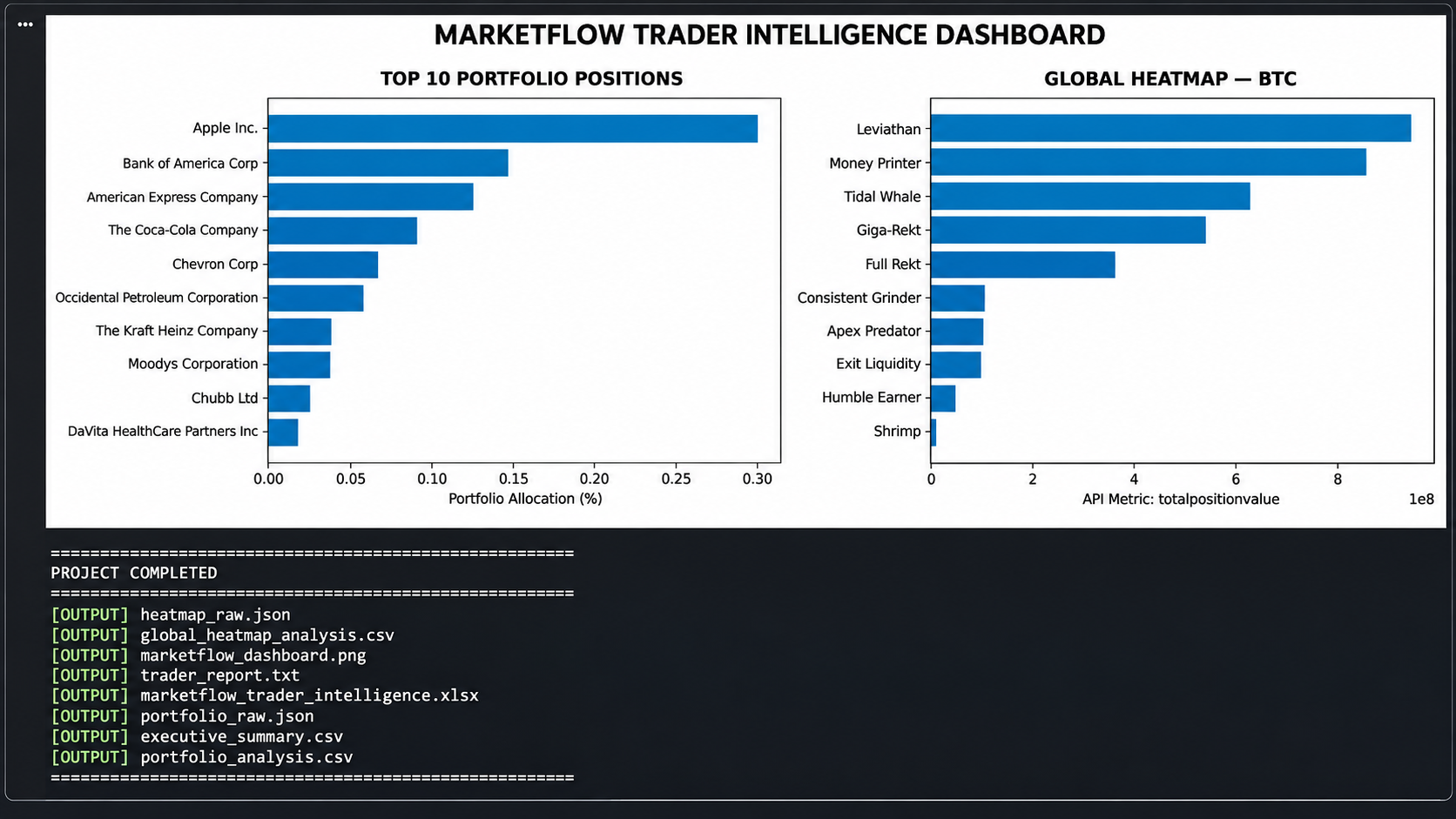
3. Results and Discussion
3.1. API Data Collection Results
The API data collection module retrieves two independent financial datasets through the MarketFlow API.
The first dataset contains portfolio information associated with Warren Buffett, using June 30, 2024, as the reporting date.
The second dataset contains global heatmap information retrieved using the BTC symbol.
Both responses are stored in JSON format before being processed into structured DataFrames.
This approach preserves the original API information and provides a foundation for examining the retrieved financial records.
The system also generates an API extraction summary that identifies whether each endpoint was successfully accessed.
3.2. Portfolio Composition and Allocation Analysis
The portfolio analysis module examines the reported holdings and identifies the fields required for portfolio allocation calculations.
The system first searches for asset identifiers, market values, portfolio weights, and holding changes.
When a portfolio weight field is available, the reported numerical values are used directly.
If the weight field is unavailable but market value exists, the system calculates estimated portfolio allocation using the proportion of each holding's market value relative to the total positive market value.
The resulting dataset is sorted in descending order of portfolio allocation.
This process enables analysts to identify the largest holdings and examine how reported portfolio exposure is distributed across different assets.
3.3. Portfolio Concentration Analysis
Portfolio concentration is evaluated using three indicators: Top 5 Concentration, Top 10 Concentration, and the Herfindahl-Hirschman Index.
Top 5 Concentration measures the combined allocation of the five largest holdings.
Top 10 Concentration measures the combined allocation of the ten largest holdings.
HHI provides a more comprehensive measurement because it incorporates the normalized allocation of every available holding.
These indicators provide complementary perspectives on portfolio structure.
A higher Top 5 Concentration indicates that a greater proportion of the portfolio is allocated to its five largest positions.
Similarly, a higher HHI indicates a more concentrated allocation structure.
The measurements should be interpreted as descriptive portfolio characteristics rather than direct indicators of investment risk or future returns.
3.4. Global Heatmap Performance Analysis
The global heatmap module examines financial instrument records returned by the API using the BTC symbol parameter.
The system identifies an asset field and a numerical performance field.
The performance field is selected using predefined keywords such as change percentage, price change, performance, return, change, and percent.
If these fields are unavailable, the framework selects the first available numerical column.
The resulting dataset is sorted in descending order, providing an overview of records with the highest and lowest numerical values.
This process allows the system to identify relative performance differences within the retrieved dataset.
However, the interpretation of the selected numerical field depends on its actual meaning and unit in the API response. For example, a raw price change, percentage change, and absolute valuation should not be interpreted interchangeably.
3.5. Market Breadth Analysis
Market breadth analysis classifies the retrieved numerical observations into positive, negative, and neutral categories.
Positive observations represent values above zero, negative observations represent values below zero, and neutral observations represent values equal to zero.
The resulting classification provides an overview of the distribution of performance values across the retrieved records.
The positive breadth calculation determines the percentage of observations with positive numerical performance.
The framework subsequently applies three descriptive classifications:
Positive breadth dominates when positive observations reach at least 60%.
Negative breadth dominates when positive observations are 40% or lower.
Mixed market breadth applies when positive observations are between 40% and 60%.
These thresholds provide a simple interpretation mechanism for the retrieved dataset.
They do not establish a statistically validated prediction of future market movements.
3.6. Trader Intelligence Interpretation
The trader interpretation module combines portfolio concentration and market breadth information.
For portfolio analysis, the system classifies Top 5 Concentration into three descriptive categories:
Top 5 Concentration | Interpretation |
|---|---|
70% or higher | Highly concentrated |
40%–below 70% | Moderately concentrated |
Below 40% | Relatively distributed |
For global market analysis, the system uses positive market breadth to determine whether the retrieved market observations demonstrate predominantly positive, predominantly negative, or mixed performance.
Combining these interpretations provides a concise overview of portfolio allocation and global heatmap performance.
Nevertheless, the results are descriptive measurements and should not be treated as direct BUY or SELL trading signals.
3.7. Financial Dashboard Visualization
The final dashboard combines two analytical visualizations into one interface.
MarketFlow Trader Intelligence Dashboard
Portfolio Distribution
Top ten holdings based on portfolio allocation.
Global Market Performance
Five highest and five lowest heatmap observations.
Dashboard composition follows the uploaded Python implementation. Actual values are populated from the API response.
The first visualization presents the ten largest portfolio positions, while the second compares the five highest and five lowest heatmap observations.
A zero reference line is included in the global performance chart to distinguish positive and negative values.
The dashboard is exported as marketflow_dashboard.png with a resolution of 200 DPI.
3.8. Exported Analytical Outputs
The framework generates eight principal output files.
Filename | Description |
|---|---|
| Original portfolio API response. |
| Original global heatmap API response. |
| Processed portfolio dataset and allocation calculations. |
| Processed heatmap dataset. |
| Summary of portfolio and market metrics. |
| Portfolio and heatmap dashboard. |
| Excel workbook containing three worksheets. |
| Consolidated financial analysis report. |
The Excel workbook contains three worksheets: Executive Summary, Portfolio Analysis, and Global Heatmap.
These files provide a structured record of the analytical workflow and allow the results to be examined using Python, Microsoft Excel, and other data analysis applications.
3.9. Analytical Limitations and Future Improvements
Several limitations should be considered when interpreting the analytical results.
First, the portfolio analysis depends on the API response structure. The system identifies fields using predefined keyword searches. If the API uses different field names, some portfolio metrics may not be calculated as expected.
Second, portfolio allocation depends on the availability of weight or market value information. If both fields are unavailable, the system cannot calculate meaningful portfolio allocation.
Third, HHI represents a descriptive concentration measurement. Its interpretation depends on the completeness of the retrieved holdings and the accuracy of the underlying portfolio weights.
Fourth, the global heatmap performance metric is selected through keyword matching. If the API does not return an explicitly identified performance field, the system uses the first available numerical column. This may not always represent percentage performance.
Fifth, the heatmap dataset is limited to the information returned by the API. The results should not automatically be interpreted as a complete representation of all global financial instruments.
Sixth, the framework does not perform predictive market analysis. It does not calculate RSI, MACD, moving averages, or future price predictions.
Seventh, the original implementation identifies a holding change field but does not use it in the final concentration or executive summary calculations. Further development could incorporate these changes into portfolio movement analysis.
Future improvements could include:
Historical portfolio comparison.
Portfolio allocation changes over multiple reporting dates.
Sector and industry concentration analysis.
Advanced HHI interpretation.
Market heatmap filtering and ranking.
Sector-based market breadth.
Relative performance comparison.
Historical market sentiment analysis.
Integration of technical indicators.
Automated financial alerts.
Portfolio risk and volatility calculations.
Predictive modeling using historical financial datasets.
These developments could expand the framework into a more comprehensive financial intelligence and portfolio monitoring platform.
4. Conclusion
This article presents the MarketFlow Trader Intelligence Analyzer, a Python-based financial analytics framework developed using the MarketFlow All-in-One Market Finance API through RapidAPI.
The system integrates Warren Buffett's portfolio information dated June 30, 2024, with global heatmap data retrieved using the BTC symbol.
The analytical workflow incorporates API authentication, financial data extraction, JSON normalization, portfolio allocation calculations, concentration measurement, global heatmap analysis, market breadth classification, and dashboard visualization.
The portfolio analysis module identifies reported holdings and evaluates their allocation through Top 5 Concentration, Top 10 Concentration, and the Herfindahl-Hirschman Index.
Meanwhile, the global heatmap module examines numerical performance observations and classifies them into positive, negative, and neutral categories.
The system also generates positive market breadth measurements and descriptive interpretations to summarize the distribution of performance values within the retrieved dataset.
The final dashboard combines the top ten portfolio positions with the highest and lowest global heatmap observations.
Additionally, the framework generates normalized CSV datasets, an executive summary, an Excel workbook, a dashboard image, and a consolidated trader intelligence report.
Overall, the MarketFlow Trader Intelligence Analyzer demonstrates how Python and financial APIs can be integrated to automate portfolio concentration analysis and global market performance monitoring.
However, the framework should be considered a descriptive financial intelligence system rather than a predictive trading platform. The accuracy of its results depends on the completeness of the API responses, the identification of appropriate numerical fields, and the interpretation of the retrieved financial information.
Future integration of historical portfolio records, sector analysis, advanced market indicators, and portfolio risk measurements could further improve the analytical capabilities of the system.