
Gold trading has become an important part of the global financial market because of its liquidity, volatility, and sensitivity to economic developments. The XAUUSD trading pair, which represents the price of gold against the US dollar, attracts traders who seek opportunities through short-term and long-term market movements. However, identifying trading opportunities requires more than observing price fluctuations. A systematic approach is needed to evaluate market trends, momentum, volatility, and potential trading risks.
Technical analysis provides several indicators that can help traders understand market conditions. Moving averages are commonly used to identify trends, the Relative Strength Index (RSI) measures momentum, the Moving Average Convergence Divergence (MACD) evaluates changes in momentum, and the Average True Range (ATR) measures market volatility. Combining these indicators can provide a structured framework for identifying potential buy and sell opportunities.
Python offers a flexible environment for developing automated trading analysis systems. Through financial APIs, historical market data can be retrieved and processed using libraries such as Requests, Pandas, and NumPy. Matplotlib can then be used to visualize price movements, technical indicators, and backtesting performance. This combination makes it possible to develop a repeatable analytical workflow without manually calculating every trading indicator.
This article presents an XAUUSD AI Trading System Using Python, a rule-based trading framework that retrieves historical gold price data from the MarketFlow All-in-One Market Finance API through RapidAPI. The system analyzes the OANDA:XAUUSD instrument using the daily timeframe and processes up to 500 historical candles.
The framework combines EMA 20, EMA 50, RSI 14, MACD, and ATR 14 to generate trading conditions. It also incorporates historical strategy backtesting, transaction-cost assumptions, equity curve comparisons, risk management, stop-loss calculations, take-profit targets, and position sizing.
The trading system is organized into five Python cells covering API configuration, historical market data acquisition, technical indicator calculation, strategy backtesting, and the final trading signal dashboard. The final output provides a BUY, SELL, or HOLD classification based on three technical confirmations.
The objective is to demonstrate how Python can integrate technical analysis, quantitative backtesting, and risk management into a structured XAUUSD trading workflow. Although the system automates calculations and signal generation, its outputs are not guaranteed predictions of future gold prices. Actual trading decisions should also consider execution costs, market conditions, broker specifications, and the possibility of losses.
2. Methodology
The XAUUSD AI Trading System uses a five-stage analytical workflow.
Cell 1 — API Configuration: imports the required libraries, establishes RapidAPI authentication, and defines trading parameters, including the instrument, timeframe, initial capital, risk percentage, risk-reward ratio, and ATR multiplier.
Cell 2 — Market Data Acquisition: retrieves historical XAUUSD price candles and attempts to retrieve IPO event information for the next 30 days.
Cell 3 — Data Processing and Technical Indicators: normalizes OHLC data and calculates EMA 20, EMA 50, RSI 14, MACD, MACD Histogram, and ATR 14.
Cell 4 — Trading Strategy and Backtesting: establishes BUY and SELL conditions, calculates strategy returns, applies transaction costs, compares strategy performance with buy-and-hold, and calculates performance metrics.
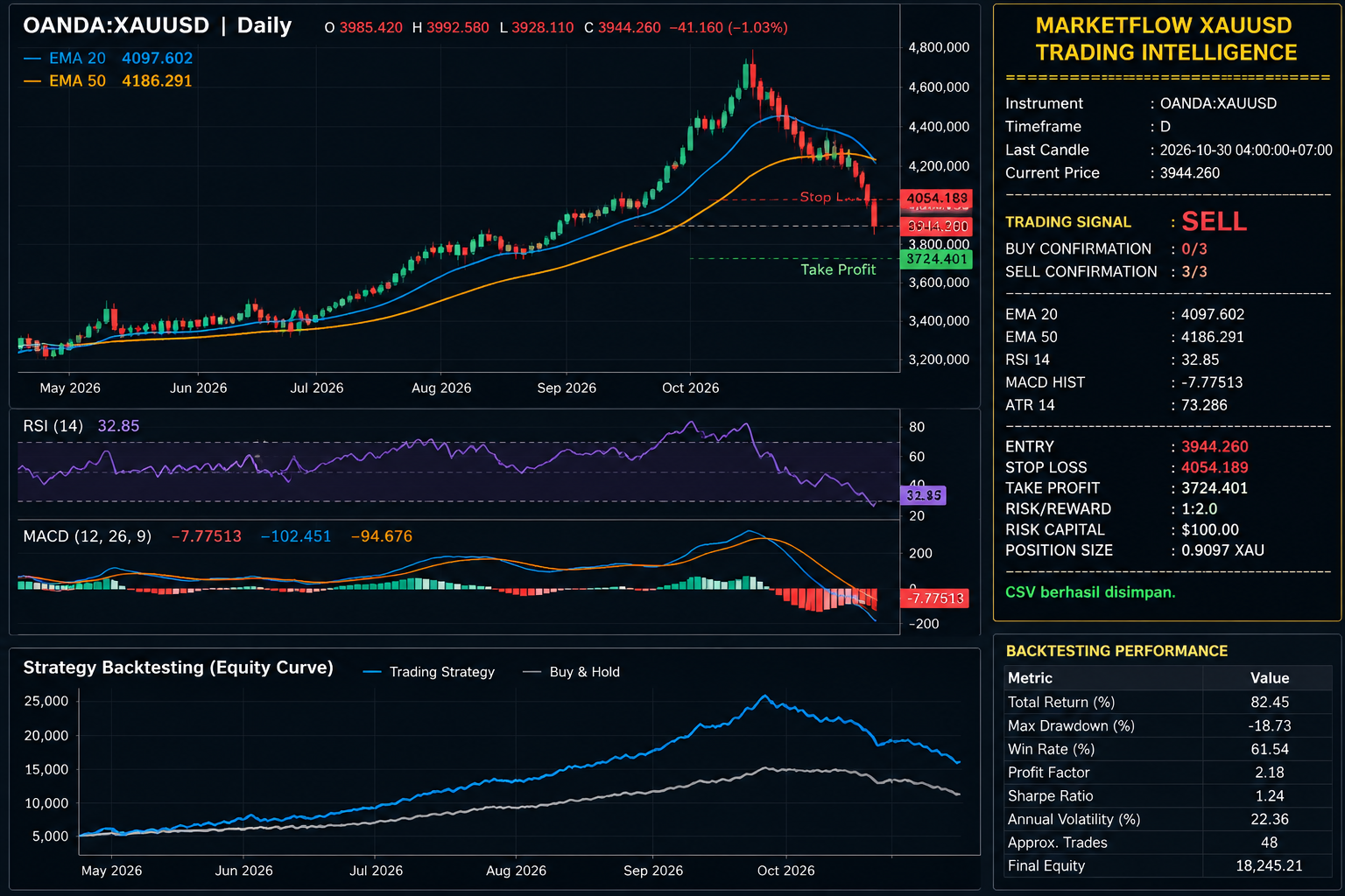
Cell 5 — Trading Signal and Risk Management Dashboard: evaluates the latest candle, calculates technical confirmations, determines the trading signal, estimates entry, stop-loss, take-profit, and position size, and exports the analytical results.
2.1. Technical Indicators
The system combines five technical indicators to evaluate market direction and momentum.
Exponential Moving Average (EMA)
EMA 20 and EMA 50 are used to identify the prevailing trend. EMA 20 represents the shorter-term trend, while EMA 50 represents the longer-term trend.
Bullish condition: EMA 20 is above EMA 50.
Bearish condition: EMA 20 is below EMA 50.
Relative Strength Index (RSI)
RSI 14 measures the strength of recent price movements on a scale from 0 to 100. The system uses RSI values between 50 and 70 for bullish confirmation and values between 30 and 50 for bearish confirmation.
Moving Average Convergence Divergence (MACD)
MACD is calculated using the difference between the 12-period and 26-period exponential moving averages. A 9-period EMA of MACD is used as its signal line.
The system evaluates the MACD Histogram:
Positive histogram: bullish momentum confirmation.
Negative histogram: bearish momentum confirmation.
Average True Range (ATR)
ATR 14 measures market volatility using the true range of each candle. It is used to estimate the distance between the entry price and stop-loss level.
2.2. Trading Signal Conditions
The trading strategy requires three simultaneous technical confirmations.
Indicator | BUY condition | SELL condition |
|---|---|---|
EMA | EMA 20 above EMA 50 | EMA 20 below EMA 50 |
RSI 14 | Above 50 and below 70 | Below 50 and above 30 |
MACD Histogram | Above 0 | Below 0 |
A BUY signal is generated when all three bullish conditions are satisfied. A SELL signal is generated when all three bearish conditions are satisfied. If neither combination is fully satisfied, the system generates a HOLD signal.
2.3. Risk Management
The system defines initial capital, percentage risk, ATR multiplier, and risk-reward ratio.
The account risk is calculated as:
\[ \text{Account Risk} = \text{Initial Capital}\times\frac{\text{Risk Percentage}}{100} \]
The stop-loss distance is calculated using:
\[ \text{Risk Distance}=\text{ATR}\times\text{ATR Multiplier} \]
The take-profit distance is then determined by:
\[ \text{Take Profit Distance}= \text{Risk Distance}\times\text{Risk Reward} \]
The position size is estimated using:
\[ \text{Position Size}= \frac{\text{Account Risk}}{\text{Risk Distance}} \]
These formulas provide an approximate position-sizing framework. Actual XAUUSD contract specifications, lot sizes, tick values, leverage, and account currency conversion must be considered before using the calculated quantity in a live trading account.
3. Implementation and Python Code
The implementation below follows the original xauusd_ai_trading_system.py file. It is divided into five cells and designed to run sequentially in Google Colab.
Cell 1 — Installation and API Configuration
The first cell imports the necessary libraries and configures the MarketFlow API connection through RapidAPI. The API key is retrieved from an environment variable or requested interactively.
The trading configuration defines XAUUSD as the instrument, uses the daily timeframe, and requests up to 500 historical candles. It also establishes the initial capital, risk percentage, risk-reward ratio, ATR multiplier, and assumed transaction cost.
These parameters control the subsequent indicator calculations, backtesting process, and risk-management dashboard.
Code — Cell 1
# ============================================================
# CELL 1 — INSTALLATION & CONFIGURATION
# ============================================================
%pip -q install requests pandas numpy matplotlib

import os, json, getpass, warnings
import requests
import numpy as np
import pandas as pd
import matplotlib.pyplot as plt

from datetime import datetime, timedelta
from IPython.display import display, Markdown

warnings.filterwarnings("ignore")

API_HOST = "marketflow-all-in-one-market-finance-api.p.rapidapi.com"
BASE_URL = f"https://{API_HOST}"

API_KEY = os.getenv("RAPIDAPI_KEY", "").strip()
if not API_KEY:
    API_KEY = getpass.getpass("Masukkan RapidAPI Key: ").strip()

if not API_KEY:
    raise ValueError("RapidAPI Key wajib diisi.")

HEADERS = {
    "x-rapidapi-key": API_KEY,
    "x-rapidapi-host": API_HOST
}

# TRADING CONFIGURATION
SYMBOL = "OANDA:XAUUSD"
TIMEFRAME = "D"
CANDLE_RANGE = 500
TIMEZONE = "Asia/Jakarta"

INITIAL_CAPITAL = 10000
RISK_PERCENT = 1.0
RISK_REWARD = 2.0
ATR_MULTIPLIER = 1.5
TRANSACTION_COST = 0.0001

def api_get(endpoint, params=None):
    response = requests.get(
        f"{BASE_URL}/{endpoint.lstrip('/')}",
        headers=HEADERS,
        params=params or {},
        timeout=30
    )
    response.raise_for_status()
    data = response.json()

    if isinstance(data, dict) and data.get("error"):
        raise RuntimeError(str(data["error"]))

    return data

print("MARKETFLOW TRADING SYSTEM READY")
print("Instrument :", SYMBOL)
print("Timeframe  :", TIMEFRAME)
print("Risk       :", f"{RISK_PERCENT}%")
Cell 2 — Historical Market Data Acquisition
The second cell retrieves historical XAUUSD price data through the /v2/chart/price endpoint. The request includes the configured candle range, timeframe, timezone, and trading symbol.
The cell also attempts to retrieve IPO event information for the next 30 days through the /ipos-events endpoint. If this endpoint is unavailable, the program stores the error in ipo_raw and continues with the historical price analysis.
The returned JSON responses are displayed in a shortened format to help inspect the API output without overwhelming the notebook.
Code — Cell 2
# ============================================================
# CELL 2 — FETCH MARKET DATA
# ============================================================

# 1. HISTORICAL XAUUSD
price_raw = api_get(
    "/v2/chart/price",
    {
        "range": CANDLE_RANGE,
        "timeframe": TIMEFRAME,
        "timezone": TIMEZONE,
        "symbol": SYMBOL
    }
)

# 2. IPO EVENTS (NEXT 30 DAYS)
today = datetime.now().date()

try:
    ipo_raw = api_get(
        "/ipos-events",
        {
            "skip": 0,
            "start_date": today.isoformat(),
            "end_date": (today + timedelta(days=30)).isoformat()
        }
    )
except Exception as e:
    ipo_raw = {"warning": str(e)}
    print("IPO endpoint tidak tersedia:", e)

print("XAUUSD API RESPONSE:")
print(json.dumps(price_raw, indent=2)[:2500])

print("\nIPO EVENTS:")
print(json.dumps(ipo_raw, indent=2)[:1500])
Cell 3 — Data Processing and Technical Indicators
The third cell processes the historical OHLC data and calculates the technical indicators required by the trading strategy.
The find_ohlc() function searches different JSON response structures for Open, High, Low, and Close data. It supports common field aliases, including open, opens, o, high, highs, h, and their corresponding low and close fields.
After extracting the price data, the program standardizes the column names, converts OHLC values into numerical formats, and identifies the available timestamp field. Timestamps are converted into the configured Jakarta timezone when they are provided in Unix format.
The system then calculates EMA 20 and EMA 50, RSI 14, MACD, MACD Signal, MACD Histogram, and ATR 14.
These indicators form the foundation of the BUY and SELL conditions evaluated in Cell 4.
Code — Cell 3
# ============================================================
# CELL 3 — DATA PROCESSING & INDICATORS
# ============================================================

def find_ohlc(obj):
    """Mencari data OHLC pada berbagai struktur JSON API."""

    aliases = {
        "open": ["open", "opens", "o"],
        "high": ["high", "highs", "h"],
        "low": ["low", "lows", "l"],
        "close": ["close", "closes", "c"],
        "time": ["timestamp", "timestamps", "time", "times", "t", "date", "datetime"]
    }

    if isinstance(obj, list):
        if obj and isinstance(obj[0], dict):
            keys = {str(k).lower() for k in obj[0].keys()}
            found = all(
                any(alias in keys for alias in aliases[k])
                for k in ["open", "high", "low", "close"]
            )
            if found:
                return pd.DataFrame(obj)

        for item in obj:
            result = find_ohlc(item)
            if result is not None:
                return result

    elif isinstance(obj, dict):
        lower = {str(k).lower(): k for k in obj.keys()}

        mapping = {}
        for standard, choices in aliases.items():
            for choice in choices:
                if choice in lower:
                    mapping[standard] = lower[choice]
                    break

        if all(k in mapping for k in ["open", "high", "low", "close"]):
            lengths = [
                len(obj[mapping[k]])
                for k in ["open", "high", "low", "close"]
                if isinstance(obj[mapping[k]], (list, tuple, np.ndarray))
            ]

            if len(lengths) == 4 and len(set(lengths)) == 1:
                return pd.DataFrame({
                    k: obj[v] for k, v in mapping.items()
                })

        for value in obj.values():
            result = find_ohlc(value)
            if result is not None:
                return result

    return None


df = find_ohlc(price_raw)

if df is None:
    raise ValueError(
        "Data OHLC tidak ditemukan. Periksa JSON response pada CELL 2."
    )

# Standardize column names
df.columns = [str(c).lower() for c in df.columns]

column_map = {}
for standard, choices in {
    "open": ["open", "opens", "o"],
    "high": ["high", "highs", "h"],
    "low": ["low", "lows", "l"],
    "close": ["close", "closes", "c"],
    "volume": ["volume", "vol", "v"]
}.items():
    for choice in choices:
        if choice in df.columns:
            column_map[choice] = standard
            break

df = df.rename(columns=column_map)

for col in ["open", "high", "low", "close"]:
    df[col] = pd.to_numeric(df[col], errors="coerce")

# Find time column
time_col = next(
    (c for c in ["time", "timestamp", "datetime", "date", "t", "times", "timestamps"]
     if c in df.columns),
    None
)

if time_col:
    timestamps = pd.to_numeric(df[time_col], errors="coerce")

    if timestamps.notna().all():
        unit = "ms" if timestamps.abs().median() > 1e11 else "s"
        df["datetime"] = pd.to_datetime(
            timestamps, unit=unit, utc=True
        ).dt.tz_convert(TIMEZONE)
    else:
        df["datetime"] = pd.to_datetime(df[time_col], errors="coerce")
else:
    df["datetime"] = pd.RangeIndex(len(df))

df = (
    df.dropna(subset=["open", "high", "low", "close"])
      .sort_values("datetime")
      .drop_duplicates("datetime")
      .reset_index(drop=True)
)

if len(df) < 60:
    raise ValueError(f"Data tidak cukup: hanya {len(df)} candle.")

# EMA
df["EMA20"] = df["close"].ewm(span=20, adjust=False).mean()
df["EMA50"] = df["close"].ewm(span=50, adjust=False).mean()

# RSI
delta = df["close"].diff()
gain = delta.clip(lower=0)
loss = -delta.clip(upper=0)

avg_gain = gain.ewm(alpha=1/14, adjust=False, min_periods=14).mean()
avg_loss = loss.ewm(alpha=1/14, adjust=False, min_periods=14).mean()

rs = avg_gain / avg_loss.replace(0, np.nan)
df["RSI"] = 100 - (100 / (1 + rs))
df.loc[(avg_loss == 0) & (avg_gain > 0), "RSI"] = 100
df.loc[(avg_loss == 0) & (avg_gain == 0), "RSI"] = 50

# MACD
ema12 = df["close"].ewm(span=12, adjust=False).mean()
ema26 = df["close"].ewm(span=26, adjust=False).mean()

df["MACD"] = ema12 - ema26
df["MACD_SIGNAL"] = df["MACD"].ewm(span=9, adjust=False).mean()
df["MACD_HIST"] = df["MACD"] - df["MACD_SIGNAL"]

# ATR
previous_close = df["close"].shift(1)

tr = pd.concat([
    df["high"] - df["low"],
    (df["high"] - previous_close).abs(),
    (df["low"] - previous_close).abs()
], axis=1).max(axis=1)

df["ATR"] = tr.ewm(alpha=1/14, adjust=False).mean()

df = df.dropna().reset_index(drop=True)

print("DATA PROCESSING COMPLETE")
print("Total candles:", len(df))
display(df.tail(10))
Cell 4 — Trading Strategy and Backtesting
The fourth cell implements the trading strategy using the technical indicators calculated in Cell 3.
The BUY condition requires EMA 20 to be above EMA 50, RSI to be between 50 and 70, and MACD Histogram to be positive. The SELL condition requires EMA 20 to be below EMA 50, RSI to be between 30 and 50, and MACD Histogram to be negative.
The strategy then generates three possible states: BUY, SELL, or HOLD. To avoid applying a signal to the same candle that generated it, the position is shifted by one candle before calculating strategy returns.
The backtesting process also includes the configured transaction cost and compares the strategy equity curve against a buy-and-hold benchmark. Performance metrics include total return, maximum drawdown, win rate, profit factor, Sharpe ratio, annualized volatility, approximate trade count, and final equity.
Code — Cell 4
# ============================================================
# CELL 4 — STRATEGY & BACKTESTING
# ============================================================

# BUY CONDITION
buy_condition = (
    (df["EMA20"] > df["EMA50"]) &
    (df["RSI"] > 50) &
    (df["RSI"] < 70) &
    (df["MACD_HIST"] > 0)
)

# SELL CONDITION
sell_condition = (
    (df["EMA20"] < df["EMA50"]) &
    (df["RSI"] < 50) &
    (df["RSI"] > 30) &
    (df["MACD_HIST"] < 0)
)

df["SIGNAL"] = np.select(
    [buy_condition, sell_condition],
    [1, -1],
    default=0
)

# BACKTEST: NEXT CANDLE POSITION
df["POSITION"] = df["SIGNAL"].shift(1).fillna(0)

# Return based on close-to-close movement
df["MARKET_RETURN"] = df["close"].pct_change().fillna(0)

# Transaction cost on position changes
df["TURNOVER"] = df["POSITION"].diff().abs()
df.loc[df.index[0], "TURNOVER"] = abs(df["POSITION"].iloc[0])

df["STRATEGY_RETURN"] = (
    df["POSITION"] * df["MARKET_RETURN"]
    - df["TURNOVER"] * TRANSACTION_COST
)

df["EQUITY"] = (
    INITIAL_CAPITAL *
    (1 + df["STRATEGY_RETURN"]).cumprod()
)

# BUY & HOLD COMPARISON
df["BUY_HOLD"] = (
    INITIAL_CAPITAL *
    (1 + df["MARKET_RETURN"]).cumprod()
)

# PERFORMANCE METRICS
returns = df["STRATEGY_RETURN"]

total_return = (df["EQUITY"].iloc[-1] / INITIAL_CAPITAL - 1) * 100

peak = df["EQUITY"].cummax()
drawdown = (df["EQUITY"] / peak) - 1
max_drawdown = drawdown.min() * 100

trades = df.loc[df["POSITION"] != 0, "STRATEGY_RETURN"]

# Daily timeframe annualization
periods = 252
annual_volatility = returns.std() * np.sqrt(periods) * 100

sharpe = (
    returns.mean() / returns.std() * np.sqrt(periods)
    if returns.std() > 0 else 0
)

gross_profit = returns[returns > 0].sum()
gross_loss = abs(returns[returns < 0].sum())

profit_factor = (
    gross_profit / gross_loss
    if gross_loss > 0 else np.inf
)

# Trade-level approximate win rate
position_change = df["POSITION"].ne(df["POSITION"].shift()).cumsum()
active = df[df["POSITION"] != 0].copy()
active["TRADE_ID"] = position_change.loc[active.index]

trade_results = (
    active.groupby("TRADE_ID")["STRATEGY_RETURN"]
    .apply(lambda x: (1 + x).prod() - 1)
)

win_rate = (
    (trade_results > 0).mean() * 100
    if len(trade_results) else 0
)

metrics = pd.DataFrame({
    "Metric": [
        "Total Return (%)",
        "Max Drawdown (%)",
        "Win Rate (%)",
        "Profit Factor",
        "Sharpe Ratio",
        "Annual Volatility (%)",
        "Approx. Trades",
        "Final Equity"
    ],
    "Value": [
        round(total_return, 2),
        round(max_drawdown, 2),
        round(win_rate, 2),
        round(profit_factor, 2) if np.isfinite(profit_factor) else "Inf",
        round(sharpe, 2),
        round(annual_volatility, 2),
        len(trade_results),
        round(df["EQUITY"].iloc[-1], 2)
    ]
})

display(metrics)

# EQUITY CURVE
plt.figure(figsize=(14, 5))
plt.plot(df["datetime"], df["EQUITY"], label="Trading Strategy")
plt.plot(df["datetime"], df["BUY_HOLD"], label="Buy & Hold", alpha=0.7)
plt.title("XAUUSD Strategy Backtesting")
plt.xlabel("Date")
plt.ylabel("Account Equity")
plt.legend()
plt.grid(alpha=0.3)
plt.show()
Cell 5 — Trading Signal and Risk Management Dashboard
The fifth cell evaluates the latest available candle and calculates the final trading signal.
The system counts three independent confirmations for BUY and SELL. When all three conditions for one direction are satisfied, the system generates the corresponding signal. Otherwise, it returns HOLD.
After determining the signal, the program calculates the entry price using the latest closing price. The ATR value is multiplied by the configured ATR multiplier to estimate the stop-loss distance. The take-profit distance is then calculated using the selected risk-reward ratio.
The position size is estimated by dividing the account risk by the stop-loss distance. The dashboard displays the instrument, timeframe, latest candle, current price, signal, technical confirmations, indicator values, and risk-management parameters.
The cell also generates a price chart containing EMA 20 and EMA 50 and exports the processed historical data and backtesting metrics to CSV files.
Code — Cell 5
# ============================================================
# CELL 5 — LIVE TRADING SIGNAL DASHBOARD
# ============================================================

last = df.iloc[-1]

price = float(last["close"])
atr = float(last["ATR"])
rsi = float(last["RSI"])

# Score based on 3 confirmations
buy_score = sum([
    last["EMA20"] > last["EMA50"],
    last["RSI"] > 50 and last["RSI"] < 70,
    last["MACD_HIST"] > 0
])

sell_score = sum([
    last["EMA20"] < last["EMA50"],
    last["RSI"] < 50 and last["RSI"] > 30,
    last["MACD_HIST"] < 0
])

if buy_score == 3:
    signal = "BUY"
elif sell_score == 3:
    signal = "SELL"
else:
    signal = "HOLD"

# ENTRY & RISK MANAGEMENT
entry = price
risk_distance = atr * ATR_MULTIPLIER
account_risk = INITIAL_CAPITAL * RISK_PERCENT / 100

if signal == "BUY":
    stop_loss = entry - risk_distance
    take_profit = entry + (risk_distance * RISK_REWARD)
elif signal == "SELL":
    stop_loss = entry + risk_distance
    take_profit = entry - (risk_distance * RISK_REWARD)
else:
    stop_loss = np.nan
    take_profit = np.nan

# Position size in XAUUSD units (approximate)
position_size = (
    account_risk / risk_distance
    if signal != "HOLD" and risk_distance > 0
    else 0
)

# Dashboard
print("=" * 55)
print("       MARKETFLOW XAUUSD TRADING INTELLIGENCE")
print("=" * 55)

print(f"Instrument       : {SYMBOL}")
print(f"Timeframe        : {TIMEFRAME}")
print(f"Last Candle      : {last['datetime']}")
print(f"Current Price    : {price:.3f}")

print("-" * 55)
print(f"TRADING SIGNAL   : {signal}")
print(f"BUY CONFIRMATION : {buy_score}/3")
print(f"SELL CONFIRMATION: {sell_score}/3")

print("-" * 55)
print(f"EMA 20           : {last['EMA20']:.3f}")
print(f"EMA 50           : {last['EMA50']:.3f}")
print(f"RSI 14           : {rsi:.2f}")
print(f"MACD HIST        : {last['MACD_HIST']:.5f}")
print(f"ATR 14           : {atr:.3f}")

print("-" * 55)

if signal != "HOLD":
    print(f"ENTRY            : {entry:.3f}")
    print(f"STOP LOSS        : {stop_loss:.3f}")
    print(f"TAKE PROFIT      : {take_profit:.3f}")
    print(f"RISK/REWARD      : 1:{RISK_REWARD}")
    print(f"RISK CAPITAL     : ${account_risk:.2f}")
    print(f"POSITION SIZE    : {position_size:.4f} XAU")
else:
    print("NO TRADE: Menunggu konfirmasi tren dan momentum.")

print("=" * 55)

# PRICE CHART
plt.figure(figsize=(15, 6))
plt.plot(df["datetime"], df["close"], label="XAUUSD Price")
plt.plot(df["datetime"], df["EMA20"], label="EMA 20")
plt.plot(df["datetime"], df["EMA50"], label="EMA 50")

plt.title(f"{SYMBOL} | {TIMEFRAME} | {signal}")
plt.xlabel("Date")
plt.ylabel("Price")
plt.legend()
plt.grid(alpha=0.3)
plt.show()

# EXPORT RESULTS
df.to_csv("XAUUSD_Trading_Analysis.csv", index=False)
metrics.to_csv("XAUUSD_Backtest_Metrics.csv", index=False)

print("CSV berhasil disimpan.")
Result:
4. Results and Discussion
4.1. Historical XAUUSD Market Data
The market-data acquisition module retrieves historical XAUUSD candles from the MarketFlow API. Each candle contains OHLC information, which represents the opening, highest, lowest, and closing prices within the selected timeframe.
The implementation requests up to 500 daily candles and converts the returned data into a standardized DataFrame. This dataset becomes the foundation for calculating technical indicators and evaluating the trading strategy.
The use of historical daily data allows the system to examine broader price movements rather than focusing exclusively on intraday fluctuations. However, the actual number of usable observations depends on the API response and the availability of valid OHLC records.
4.2. Technical Indicator Analysis
The technical indicator module combines trend, momentum, and volatility measurements.
EMA 20 and EMA 50 establish the trend direction. When EMA 20 is above EMA 50, the system recognizes a bullish trend condition. When EMA 20 is below EMA 50, it recognizes a bearish trend condition.
RSI 14 provides momentum confirmation. The strategy avoids treating extremely high RSI values above 70 as bullish confirmation and avoids treating values below 30 as bearish confirmation. This creates a more selective entry condition.
The MACD Histogram provides another momentum filter. Positive values support the BUY condition, while negative values support the SELL condition.
ATR 14 complements these indicators by measuring market volatility. Its value is used to estimate the stop-loss distance and calculate the corresponding take-profit level.
Combining these indicators allows the system to require agreement between trend direction and momentum before generating a directional signal.
4.3. Trading Signal Generation
The signal-generation module evaluates the latest available candle using three technical confirmations.
A BUY signal requires:
EMA 20 above EMA 50.
RSI between 50 and 70.
MACD Histogram above zero.
A SELL signal requires:
EMA 20 below EMA 50.
RSI between 30 and 50.
MACD Histogram below zero.
When all three conditions for one direction are satisfied, the system generates the corresponding signal. If the conditions are incomplete or conflicting, the system returns HOLD.
The confirmation score provides additional information about the signal. For example, a BUY confirmation of 3/3 indicates that all three bullish conditions are satisfied.
Nevertheless, a complete confirmation score does not guarantee that the next price movement will follow the expected direction. Technical indicators are derived from historical price data and may respond with a delay when market conditions change rapidly.
4.4. Backtesting and Strategy Performance
The backtesting module evaluates the historical performance of the trading conditions using the available XAUUSD candles.
The position generated by each signal is shifted by one candle. This means the strategy uses the previous candle's signal when calculating the current candle's return, rather than applying the signal to the same candle that generated it.
The strategy equity curve is calculated by compounding the strategy returns from the initial capital. A buy-and-hold equity curve is also generated as a comparison benchmark.
The framework calculates several performance metrics:
Metric | Analytical purpose |
|---|---|
Total Return | Measures cumulative strategy performance. |
Maximum Drawdown | Measures the largest decline from a previous equity peak. |
Win Rate | Estimates the percentage of profitable grouped positions. |
Profit Factor | Compares gross positive returns with gross negative returns. |
Sharpe Ratio | Evaluates average returns relative to return volatility. |
Annual Volatility | Estimates annualized return variability. |
Approximate Trades | Counts grouped periods of active positions. |
Final Equity | Reports the ending simulated account value. |
These metrics provide different perspectives on historical performance. A strategy may generate positive total returns but still experience substantial drawdowns. Similarly, a high win rate does not necessarily imply profitability if the average losing trade is substantially larger than the average winning trade.
The results should therefore be evaluated collectively rather than relying on a single performance metric.
4.5. Stop-Loss, Take-Profit, and Position Sizing
The risk-management dashboard uses ATR 14 to estimate the distance between entry and stop-loss levels.
With an ATR multiplier of 1.5 and a risk-reward ratio of 1:2, the system establishes a take-profit distance equal to twice the estimated stop-loss distance.
The initial capital is configured at $10,000, with a risk allocation of 1% per trade. This produces a nominal account risk budget of $100.
The estimated position size is calculated by dividing the risk budget by the stop-loss distance. This calculation provides a simplified quantity estimate based on the instrument's price movement.
However, the resulting position size is not automatically equivalent to a broker-supported lot size. XAUUSD contract specifications, tick values, minimum volume, margin requirements, and account currency must be checked before using the quantity for actual trading.
4.6. Limitations and Future Improvements
Several limitations should be considered when interpreting the results.
First, the system is rule-based rather than a machine-learning model. Although it is titled an AI Trading System, the current implementation uses predefined technical conditions. It does not train a predictive model or learn trading patterns from historical observations.
Second, the IPO event data are not integrated into the trading strategy. The program retrieves upcoming IPO information, but the returned events are not used to modify the XAUUSD signals. Consequently, the trading decisions depend entirely on the technical indicators.
Third, the backtesting model is simplified. It uses close-to-close returns, shifted positions, and a fixed transaction-cost assumption. It does not simulate bid-ask spreads, slippage, financing charges, stop-loss execution, take-profit execution, or intrabar price movements.
Fourth, position sizing is approximate. The calculation assumes that the price-distance-based quantity directly corresponds to the account's monetary risk. Actual XAUUSD contract specifications may produce different risk exposure.
Fifth, the strategy uses historical data from a limited observation window. Although 500 daily candles provide a useful starting point, additional historical periods and out-of-sample testing are necessary to evaluate whether the strategy performs consistently under different market conditions.
Future improvements could include walk-forward testing, parameter optimization, volatility-adjusted position sizing, realistic execution simulations, economic-calendar integration, and machine-learning-based signal evaluation.
These improvements would help transform the current analytical framework into a more comprehensive quantitative trading research system.
5. Conclusion
The XAUUSD AI Trading System demonstrates how Python can integrate financial API connectivity, historical price analysis, technical indicators, strategy backtesting, and risk management into a single analytical workflow.
The implementation combines EMA 20, EMA 50, RSI 14, MACD Histogram, and ATR 14 to evaluate market conditions and generate BUY, SELL, or HOLD signals. It also calculates historical strategy performance, compares the resulting equity curve with a buy-and-hold benchmark, and estimates entry, stop-loss, take-profit, and position-size parameters.
The five-cell structure makes the system suitable for systematic experimentation in Google Colab. Each stage performs a distinct function, from retrieving market data to generating the final trading dashboard and exporting analytical results.
Nevertheless, the reliability of the trading system depends on historical data quality, parameter selection, realistic transaction-cost assumptions, and proper interpretation of the backtesting metrics. A technically confirmed signal should not be considered a guaranteed prediction of future market movements.
Future development should focus on more realistic backtesting, broker-specific position sizing, out-of-sample validation, and additional market-context analysis. With these improvements, the framework can serve as a foundation for quantitative XAUUSD trading research and the development of more advanced automated trading systems.