
Financial and commodity markets require a systematic approach because price movements alone do not provide sufficient information for making a trading decision. A more robust analysis combines trend structure, momentum, volatility, directional strength, support and resistance, and predefined risk management rules. This project develops a MarketFlow Trading Intelligence Engine that analyzes XAUUSD and BTCUSDT using daily market data retrieved through the MarketFlow API.
The system processes up to 100 daily candles for each selected asset and converts the raw API response into a standardized OHLCV dataset. It then calculates several technical indicators, including EMA20, EMA50, RSI14, MACD, ATR14, ADX14, +DI, -DI, 20-period support, 20-period resistance, and annualized 20-period volatility. These indicators are combined into a rule-based signal engine. marketflow_trading_intelligence marketflow_trading_intelligence
The trading engine does not rely on a single indicator. A LONG decision requires five bullish confirmations: bullish EMA structure, positive MACD histogram, RSI between 50 and 70, ADX of at least 25, and +DI greater than -DI. A SHORT decision applies the corresponding bearish conditions. If all five conditions are not satisfied, the system returns WAIT rather than forcing a trade. marketflow_trading_intelligence
The system also incorporates ATR-based risk management. The stop-loss distance is calculated from ATR multiplied by a predefined multiplier of 1.5. Two profit targets are generated at 1.5R and 2.5R. Position quantity is estimated from the account risk budget divided by the ATR-based risk distance. marketflow_trading_intelligence
Cell 1 — Library & API Configuration
The first cell prepares the Python environment and defines the MarketFlow API connection. Pandas is used for tabular data processing, NumPy for numerical calculations, Matplotlib and mplfinance for visualization, Requests for API communication, and IPython Display for presenting DataFrames.
The system analyzes two assets:
XAUUSD, retrieved from OANDA through
/v2/chart/priceBTCUSDT, retrieved from Binance through
/v2/chart/historical
Both assets use a daily timeframe with a 100-candle range. The trading configuration uses a USD 10,000 account balance, 1% risk per trade, an ATR stop multiplier of 1.5, and two reward-to-risk targets of 1.5R and 2.5R. marketflow_trading_intelligence
Code
# ============================================================
# CELL 1 — LIBRARY & CONFIGURATION
# ============================================================

%pip -q install requests pandas numpy matplotlib mplfinance

import requests
import pandas as pd
import numpy as np
import matplotlib.pyplot as plt
import mplfinance as mpf
import warnings
from IPython.display import display

warnings.filterwarnings("ignore")

HOST = "marketflow-all-in-one-market-finance-api.p.rapidapi.com"
BASE_URL = f"https://{HOST}"

# Isi dengan RapidAPI key Anda
API_KEY = "YOUR_API_KEY"

HEADERS = {
    "x-rapidapi-key": API_KEY,
    "x-rapidapi-host": HOST
}

ASSETS = {
    "XAUUSD": {
        "symbol": "OANDA:XAUUSD",
        "endpoint": "/v2/chart/price",
        "params": {
            "range": 100,
            "timeframe": "D",
            "timezone": "Asia/Jakarta"
        }
    },
    "BTCUSDT": {
        "symbol": "BINANCE:BTCUSDT",
        "endpoint": "/v2/chart/historical",
        "params": {
            "range": 100,
            "timeframe": "D",
            "to": "2025-12-31",
            "timezone": "Asia/Jakarta"
        }
    }
}

ACCOUNT_BALANCE = 10000.0  # USD, contoh untuk sizing
RISK_PERCENT = 1.0
ATR_STOP_MULTIPLIER = 1.5
RR_TARGET_1 = 1.5
RR_TARGET_2 = 2.5

print("=" * 65)
print("MARKETFLOW TRADING INTELLIGENCE ENGINE")
print("=" * 65)
print("Assets       :", list(ASSETS))
print("Timeframe    : Daily")
print("Candle Range : 100")
print("Risk / Trade :", f"{RISK_PERCENT}%")
print("Status       : Configuration ready")
Cell 1 therefore establishes the analytical environment and the assumptions that control the rest of the system. The use of explicit risk parameters is important because the system does not treat every potential trade as having the same risk profile.
Cell 2 — Market Data Fetch & Normalization
The second cell retrieves OHLCV data from the MarketFlow API and converts different possible response structures into a single standardized DataFrame.
The normalization process is deliberately flexible. It recognizes alternative names such as timestamp, datetime, date, o, h, l, c, and vol. It also handles both dictionary-based records and list-based OHLCV arrays.
The timestamps are converted into UTC and then Jakarta time. Duplicate timestamps are removed, invalid OHLC relationships are filtered, and at least 60 candles are required before the dataset is accepted. marketflow_trading_intelligence marketflow_trading_intelligence
Code
# ============================================================
# CELL 2 — MARKET DATA FETCH & NORMALIZATION
# ============================================================

def fetch_market_data(config):
    params = {
        **config["params"],
        "symbol": config["symbol"]
    }

    response = requests.get(
        BASE_URL + config["endpoint"],
        headers=HEADERS,
        params=params,
        timeout=30
    )

    print(
        f"{config['symbol']} | HTTP {response.status_code}"
    )
    response.raise_for_status()
    return response.json()


def normalize_ohlcv(payload):
    aliases = {
        "time": ["time", "timestamp", "datetime", "date", "t"],
        "open": ["open", "o"],
        "high": ["high", "h"],
        "low": ["low", "l"],
        "close": ["close", "c"],
        "volume": ["volume", "vol", "v"]
    }

    def standardize(frame):
        frame = frame.copy()
        frame.columns = [str(c).lower() for c in frame.columns]

        rename = {}
        for target, keys in aliases.items():
            for key in keys:
                if key in frame.columns:
                    rename[key] = target
                    break

        frame = frame.rename(columns=rename)

        required = ["time", "open", "high", "low", "close"]
        if not all(k in frame.columns for k in required):
            return None

        if "volume" not in frame.columns:
            frame["volume"] = np.nan

        numeric = ["open", "high", "low", "close", "volume"]
        for col in numeric:
            frame[col] = pd.to_numeric(
                frame[col], errors="coerce"
            )

        ts = frame["time"]

        if pd.api.types.is_numeric_dtype(ts):
            vals = pd.to_numeric(ts, errors="coerce")
            unit = "ms" if vals.dropna().abs().median() > 1e11 else "s"
            frame["time"] = pd.to_datetime(
                vals, unit=unit, utc=True, errors="coerce"
            ).dt.tz_convert("Asia/Jakarta")
        else:
            parsed = pd.to_datetime(ts, errors="coerce")

            if parsed.dt.tz is None:
                parsed = parsed.dt.tz_localize(
                    "Asia/Jakarta",
                    ambiguous="NaT",
                    nonexistent="NaT"
                )
            else:
                parsed = parsed.dt.tz_convert("Asia/Jakarta")

            frame["time"] = parsed

        frame = (
            frame.dropna(subset=required)
            .sort_values("time")
            .drop_duplicates("time")
            .set_index("time")
        )

        valid = (
            (frame["high"] >= frame[["open", "close", "low"]].max(axis=1)) &
            (frame["low"] <= frame[["open", "close", "high"]].min(axis=1)) &
            (frame["low"] > 0)
        )
        frame = frame.loc[valid]

        return frame[["open", "high", "low", "close", "volume"]]

    def walk(obj):
        if isinstance(obj, list):
            if obj and all(isinstance(x, dict) for x in obj):
                result = standardize(pd.DataFrame(obj))
                if result is not None and len(result):
                    return result

            if obj and all(
                isinstance(x, (list, tuple)) and len(x) >= 5
                for x in obj
            ):
                width = min(len(obj[0]), 6)
                cols = ["time", "open", "high", "low", "close", "volume"]
                result = standardize(
                    pd.DataFrame([x[:width] for x in obj],
                                 columns=cols[:width])
                )
                if result is not None and len(result):
                    return result

            for item in obj:
                result = walk(item)
                if result is not None:
                    return result

        if isinstance(obj, dict):
            lower = {str(k).lower(): v for k, v in obj.items()}

            # Columnar format, e.g. {"t":[], "o":[], ...}
            if all(k in lower for k in ["t", "o", "h", "l", "c"]):
                result = standardize(pd.DataFrame(lower))
                if result is not None and len(result):
                    return result

            if all(k in lower for k in
                   ["time", "open", "high", "low", "close"]):
                if all(isinstance(lower[k], list) for k in
                       ["time", "open", "high", "low", "close"]):
                    result = standardize(pd.DataFrame(lower))
                    if result is not None and len(result):
                        return result

            for value in obj.values():
                result = walk(value)
                if result is not None:
                    return result

        return None

    result = walk(payload)

    if result is None or result.empty:
        raise ValueError(
            "OHLCV tidak ditemukan. Periksa struktur respons API."
            f"\nPreview: {str(payload)[:800]}"
        )

    return result


market_data = {}
errors = {}

for asset, config in ASSETS.items():
    try:
        raw = fetch_market_data(config)
        df = normalize_ohlcv(raw)

        if len(df) < 60:
            raise ValueError(
                f"Candle tidak cukup: {len(df)} (minimum 60)"
            )

        market_data[asset] = df

        print(
            f"SUCCESS | {asset} | {len(df)} candles | "
            f"{df.index[-1]}"
        )
        display(df.tail(3))

    except Exception as e:
        errors[asset] = str(e)
        print(f"FAILED | {asset} | {e}")

print("\nAvailable datasets:", list(market_data))
Tahap normalisasi ini sangat penting karena kualitas indikator teknikal bergantung langsung pada kualitas OHLCV. Sistem tidak langsung menghitung indikator dari respons mentah API. Data terlebih dahulu disortir, diduplikasi, dikonversi, dan divalidasi.
Cell 3 — Technical Indicator Engine
Cell 3 merupakan inti analisis teknikal. Fungsi calculate_indicators() menghasilkan beberapa kelompok indikator.
Trend structure
\[ EMA20 \]
dan
\[ EMA50 \]
digunakan untuk menentukan struktur tren jangka pendek dan menengah.
Momentum
RSI14 digunakan untuk membedakan momentum bullish dan bearish. MACD dibentuk dari EMA12 dan EMA26, kemudian MACD signal menggunakan EMA9.
Volatility
ATR14 digunakan untuk mengukur volatilitas absolut, sedangkan ATR_PERCENT menunjukkan ATR relatif terhadap harga.
Trend strength
ADX14 bersama PLUS_DI dan MINUS_DI digunakan untuk mengukur kekuatan dan arah tren.
Market structure
Support dan resistance dihitung dari minimum low dan maksimum high pada 20 candle sebelumnya, dengan menggunakan .shift(1) sehingga candle saat ini tidak masuk ke dalam level tersebut. marketflow_trading_intelligence
Code
# ============================================================
# CELL 3 — TECHNICAL INDICATOR ENGINE
# ============================================================

def calculate_indicators(df):
    d = df.copy()

    close = d["close"]
    high = d["high"]
    low = d["low"]

    # Exponential Moving Averages
    d["EMA20"] = close.ewm(
        span=20, adjust=False
    ).mean()

    d["EMA50"] = close.ewm(
        span=50, adjust=False
    ).mean()

    # RSI 14 - Wilder smoothing
    delta = close.diff()
    gain = delta.clip(lower=0)
    loss = -delta.clip(upper=0)

    avg_gain = gain.ewm(
        alpha=1/14, adjust=False, min_periods=14
    ).mean()

    avg_loss = loss.ewm(
        alpha=1/14, adjust=False, min_periods=14
    ).mean()

    rs = avg_gain / avg_loss.replace(0, np.nan)
    d["RSI"] = 100 - (100 / (1 + rs))
    d.loc[(avg_loss == 0) & (avg_gain > 0), "RSI"] = 100
    d.loc[(avg_gain == 0) & (avg_loss > 0), "RSI"] = 0
    d.loc[(avg_gain == 0) & (avg_loss == 0), "RSI"] = 50

    # MACD
    ema12 = close.ewm(span=12, adjust=False).mean()
    ema26 = close.ewm(span=26, adjust=False).mean()

    d["MACD"] = ema12 - ema26
    d["MACD_SIGNAL"] = d["MACD"].ewm(
        span=9, adjust=False
    ).mean()
    d["MACD_HIST"] = d["MACD"] - d["MACD_SIGNAL"]

    # True Range & ATR
    tr = pd.concat([
        high - low,
        (high - close.shift()).abs(),
        (low - close.shift()).abs()
    ], axis=1).max(axis=1)

    d["ATR"] = tr.ewm(
        alpha=1/14, adjust=False, min_periods=14
    ).mean()

    d["ATR_PERCENT"] = d["ATR"] / close * 100

    # Directional Movement & ADX
    up = high.diff()
    down = -low.diff()

    plus_dm = pd.Series(
        np.where((up > down) & (up > 0), up, 0.0),
        index=d.index
    )
    minus_dm = pd.Series(
        np.where((down > up) & (down > 0), down, 0.0),
        index=d.index
    )

    smooth_tr = tr.ewm(
        alpha=1/14, adjust=False, min_periods=14
    ).mean()

    plus_di = 100 * (
        plus_dm.ewm(alpha=1/14, adjust=False,
                    min_periods=14).mean() / smooth_tr
    )

    minus_di = 100 * (
        minus_dm.ewm(alpha=1/14, adjust=False,
                     min_periods=14).mean() / smooth_tr
    )

    dx = 100 * (
        (plus_di - minus_di).abs() /
        (plus_di + minus_di).replace(0, np.nan)
    )

    d["ADX"] = dx.ewm(
        alpha=1/14, adjust=False, min_periods=14
    ).mean()

    d["PLUS_DI"] = plus_di
    d["MINUS_DI"] = minus_di

    # Prior 20 completed candles
    d["SUPPORT20"] = low.shift(1).rolling(20).min()
    d["RESISTANCE20"] = high.shift(1).rolling(20).max()

    d["RETURN_PCT"] = close.pct_change() * 100
    d["VOLATILITY20"] = (
        d["RETURN_PCT"].rolling(20).std() * np.sqrt(365)
    )

    return d


analysis_data = {}

for asset, df in market_data.items():
    result = calculate_indicators(df)
    analysis_data[asset] = result

    print("\n" + "=" * 65)
    print("TECHNICAL ANALYSIS:", asset)
    print("=" * 65)

    cols = [
        "close", "EMA20", "EMA50",
        "RSI", "MACD_HIST", "ATR",
        "ADX", "SUPPORT20", "RESISTANCE20"
    ]

    display(result[cols].tail(5).round(3))
Dengan struktur ini, sistem tidak hanya melihat arah harga. Ia mengevaluasi trend, momentum, volatility, directional strength, dan market structure secara bersamaan.
Cell 4 — Signal Engine & Trade Management
Cell 4 mengubah indikator menjadi keputusan trading.
Untuk LONG, lima kondisi harus terpenuhi:
Price > EMA20 > EMA50MACD_HIST > 050 < RSI < 70ADX >= 25PLUS_DI > MINUS_DI
Untuk SHORT:
Price < EMA20 < EMA50MACD_HIST < 030 < RSI < 50ADX >= 25MINUS_DI > PLUS_DI
Semua lima konfirmasi harus terpenuhi. Jika hanya empat, tiga, atau kurang yang terpenuhi, sistem menghasilkan WAIT. marketflow_trading_intelligence
Confidence atau rule score dihitung sebagai:
\[ Confidence = \frac{\max(LongScore, ShortScore)}{5} \times 100 \]
Stop-loss menggunakan:
\[ RiskDistance = ATR \times 1.5 \]
Untuk LONG:
\[ SL = Entry - RiskDistance \]\[ TP1 = Entry + 1.5(RiskDistance) \]\[ TP2 = Entry + 2.5(RiskDistance) \]
Untuk SHORT arah perhitungannya dibalik. Position quantity kemudian dihitung berdasarkan risk budget akun. marketflow_trading_intelligence
Code
# ============================================================
# CELL 4 — SIGNAL ENGINE & TRADE MANAGEMENT
# ============================================================

def generate_signal(asset, df):
    d = df.dropna(subset=[
        "EMA20", "EMA50", "RSI", "ATR",
        "ADX", "MACD_HIST", "SUPPORT20", "RESISTANCE20"
    ])

    if d.empty:
        return {
            "Asset": asset,
            "Signal": "WAIT",
            "Reason": "Insufficient indicator data"
        }

    x = d.iloc[-1]
    price = float(x["close"])
    atr = float(x["ATR"])

    trend_up = (
        price > x["EMA20"] > x["EMA50"]
    )
    trend_down = (
        price < x["EMA20"] < x["EMA50"]
    )

    macd_up = x["MACD_HIST"] > 0
    macd_down = x["MACD_HIST"] < 0

    rsi_up = 50 < x["RSI"] < 70
    rsi_down = 30 < x["RSI"] < 50

    strong_trend = x["ADX"] >= 25
    di_up = x["PLUS_DI"] > x["MINUS_DI"]
    di_down = x["MINUS_DI"] > x["PLUS_DI"]

    long_checks = [
        bool(trend_up),
        bool(macd_up),
        bool(rsi_up),
        bool(strong_trend),
        bool(di_up)
    ]

    short_checks = [
        bool(trend_down),
        bool(macd_down),
        bool(rsi_down),
        bool(strong_trend),
        bool(di_down)
    ]

    long_score = sum(long_checks)
    short_score = sum(short_checks)

    # All five confirmations required
    if long_score == 5:
        signal = "LONG"
        reason = "Bullish confirmations aligned"

    elif short_score == 5:
        signal = "SHORT"
        reason = "Bearish confirmations aligned"

    else:
        signal = "WAIT"
        reason = "Technical confirmations incomplete"

    dominant_score = max(long_score, short_score)
    confidence = dominant_score / 5 * 100

    # ATR-based trade setup
    risk_distance = atr * ATR_STOP_MULTIPLIER

    entry = price if signal != "WAIT" else np.nan

    if signal == "LONG":
        stop = entry - risk_distance
        tp1 = entry + risk_distance * RR_TARGET_1
        tp2 = entry + risk_distance * RR_TARGET_2

    elif signal == "SHORT":
        stop = entry + risk_distance
        tp1 = entry - risk_distance * RR_TARGET_1
        tp2 = entry - risk_distance * RR_TARGET_2

    else:
        stop = tp1 = tp2 = np.nan

    risk_usd = ACCOUNT_BALANCE * RISK_PERCENT / 100

    # Quantity in base asset / XAU ounces
    # Does not include contract multipliers, fees or slippage
    quantity = (
        risk_usd / risk_distance
        if signal != "WAIT" and risk_distance > 0
        else np.nan
    )

    return {
        "Asset": asset,
        "Candle Time": str(d.index[-1]),
        "Price": price,
        "Trend": (
            "BULLISH" if trend_up else
            "BEARISH" if trend_down else "MIXED"
        ),
        "RSI": round(x["RSI"], 2),
        "ADX": round(x["ADX"], 2),
        "ATR": round(atr, 4),
        "Support": round(x["SUPPORT20"], 4),
        "Resistance": round(x["RESISTANCE20"], 4),
        "Signal": signal,
        "Rule Score %": confidence,
        "Entry": entry,
        "Stop Loss": stop,
        "Take Profit 1": tp1,
        "Take Profit 2": tp2,
        "RR TP1": RR_TARGET_1 if signal != "WAIT" else np.nan,
        "RR TP2": RR_TARGET_2 if signal != "WAIT" else np.nan,
        "Risk USD": risk_usd if signal != "WAIT" else np.nan,
        "Quantity": quantity,
        "Reason": reason
    }


signals = []

for asset, df in analysis_data.items():
    signals.append(generate_signal(asset, df))

report = pd.DataFrame(signals)

print("=" * 85)
print("FINAL TRADING INTELLIGENCE REPORT")
print("=" * 85)

display(report.round(4))

for _, row in report.iterrows():
    print("\n" + "-" * 65)
    print(f"ASSET       : {row['Asset']}")
    print(f"CANDLE      : {row['Candle Time']}")
    print(f"PRICE       : {row['Price']:,.4f}")
    print(f"TREND       : {row['Trend']}")
    print(f"SIGNAL      : {row['Signal']}")
    print(f"RULE SCORE  : {row['Rule Score %']:.0f}%")
    print(f"REASON      : {row['Reason']}")

    if row["Signal"] != "WAIT":
        print(f"ENTRY       : {row['Entry']:,.4f}")
        print(f"STOP LOSS   : {row['Stop Loss']:,.4f}")
        print(f"TARGET 1    : {row['Take Profit 1']:,.4f}")
        print(f"TARGET 2    : {row['Take Profit 2']:,.4f}")
        print(f"RISK        : ${row['Risk USD']:,.2f}")
        print(f"QUANTITY    : {row['Quantity']:.6f}")
    else:
        print("ACTION      : No trade setup")
Sistem ini menggunakan pendekatan all-confirmation, bukan weighted scoring. Artinya, rule score 80% tidak otomatis menghasilkan trade. Hanya score 100% untuk sisi LONG atau SHORT yang dapat menghasilkan sinyal tersebut. Ini merupakan karakteristik penting dari model keputusan pada source code. marketflow_trading_intelligence
Cell 5 — Trading Dashboard & Export
Cell terakhir menyediakan visualisasi dan ekspor hasil.
Untuk setiap aset, sistem mengambil 80 candle terakhir dan menampilkan:
Candlestick price
EMA20
EMA50
Support20
Resistance20
RSI
MACD Histogram
Jika sinyal LONG atau SHORT tersedia, entry, stop-loss, TP1, dan TP2 juga ditambahkan ke chart.
Setiap chart disimpan sebagai file PNG dengan nama berdasarkan aset, sedangkan hasil keseluruhan disimpan sebagai marketflow_trading_report.csv. Data indikator setiap aset juga diekspor ke file CSV terpisah. marketflow_trading_intelligence
Code
# ============================================================
# CELL 5 — TRADING DASHBOARD & EXPORT
# ============================================================

for asset, df in analysis_data.items():

    d = df.tail(80).copy()

    if d.empty:
        continue

    info = report.loc[report["Asset"] == asset].iloc[0]

    # Convert index to mplfinance-compatible datetime
    chart = d.copy()
    chart.index = chart.index.tz_localize(None)

    volume_available = (
        chart["volume"].notna().all()
        and (chart["volume"] >= 0).all()
    )

    overlays = [
        mpf.make_addplot(
            chart["EMA20"], color="dodgerblue", width=1.3
        ),
        mpf.make_addplot(
            chart["EMA50"], color="orange", width=1.3
        ),
        mpf.make_addplot(
            chart["SUPPORT20"],
            color="green", linestyle="--", width=0.8
        ),
        mpf.make_addplot(
            chart["RESISTANCE20"],
            color="red", linestyle="--", width=0.8
        ),
        mpf.make_addplot(
            chart["RSI"],
            panel=1, color="purple", ylabel="RSI"
        ),
        mpf.make_addplot(
            chart["MACD_HIST"],
            panel=2, type="bar",
            color="steelblue", ylabel="MACD Hist"
        )
    ]

    price_lines = []

    if info["Signal"] != "WAIT":
        price_lines = [
            info["Entry"],
            info["Stop Loss"],
            info["Take Profit 1"],
            info["Take Profit 2"]
        ]

    settings = dict(
        type="candle",
        style="yahoo",
        addplot=overlays,
        volume=False,
        figsize=(16, 10),
        panel_ratios=(5, 2, 2),
        title=(
            f"\n{asset} | DAILY TRADING ANALYSIS | "
            f"{info['Signal']} | "
            f"Rule Score: {info['Rule Score %']:.0f}%\n"
        ),
        ylabel="Price (USD)",
        tight_layout=True,
        returnfig=True
    )

    if price_lines:
        settings["hlines"] = dict(
            hlines=price_lines,
            colors=["blue", "red", "green", "darkgreen"],
            linestyle="--",
            linewidths=1
        )

    fig, axes = mpf.plot(chart, **settings)

    fig.savefig(
        f"{asset}_trading_analysis.png",
        dpi=180,
        bbox_inches="tight"
    )

    plt.show()
    plt.close(fig)

    print(f"\n{'=' * 65}")
    print(f"TRADE DECISION — {asset}")
    print(f"{'=' * 65}")
    print(f"Signal     : {info['Signal']}")
    print(f"Trend      : {info['Trend']}")
    print(f"Rule Score : {info['Rule Score %']:.0f}%")
    print(f"RSI        : {info['RSI']:.2f}")
    print(f"ADX        : {info['ADX']:.2f}")
    print(f"Support    : {info['Support']:,.4f}")
    print(f"Resistance : {info['Resistance']:,.4f}")
    print(f"Reason     : {info['Reason']}")

    if info["Signal"] != "WAIT":
        print(f"Entry      : {info['Entry']:,.4f}")
        print(f"Stop Loss  : {info['Stop Loss']:,.4f}")
        print(f"TP1        : {info['Take Profit 1']:,.4f}")
        print(f"TP2        : {info['Take Profit 2']:,.4f}")
    else:
        print("Decision   : WAIT — no qualifying trade")

# Export
report.to_csv(
    "marketflow_trading_report.csv",
    index=False
)

for asset, df in analysis_data.items():
    df.to_csv(f"{asset}_indicators.csv")

print("\nEXPORT COMPLETED")
print("marketflow_trading_report.csv")
print("Individual asset charts and indicator CSV files saved.")
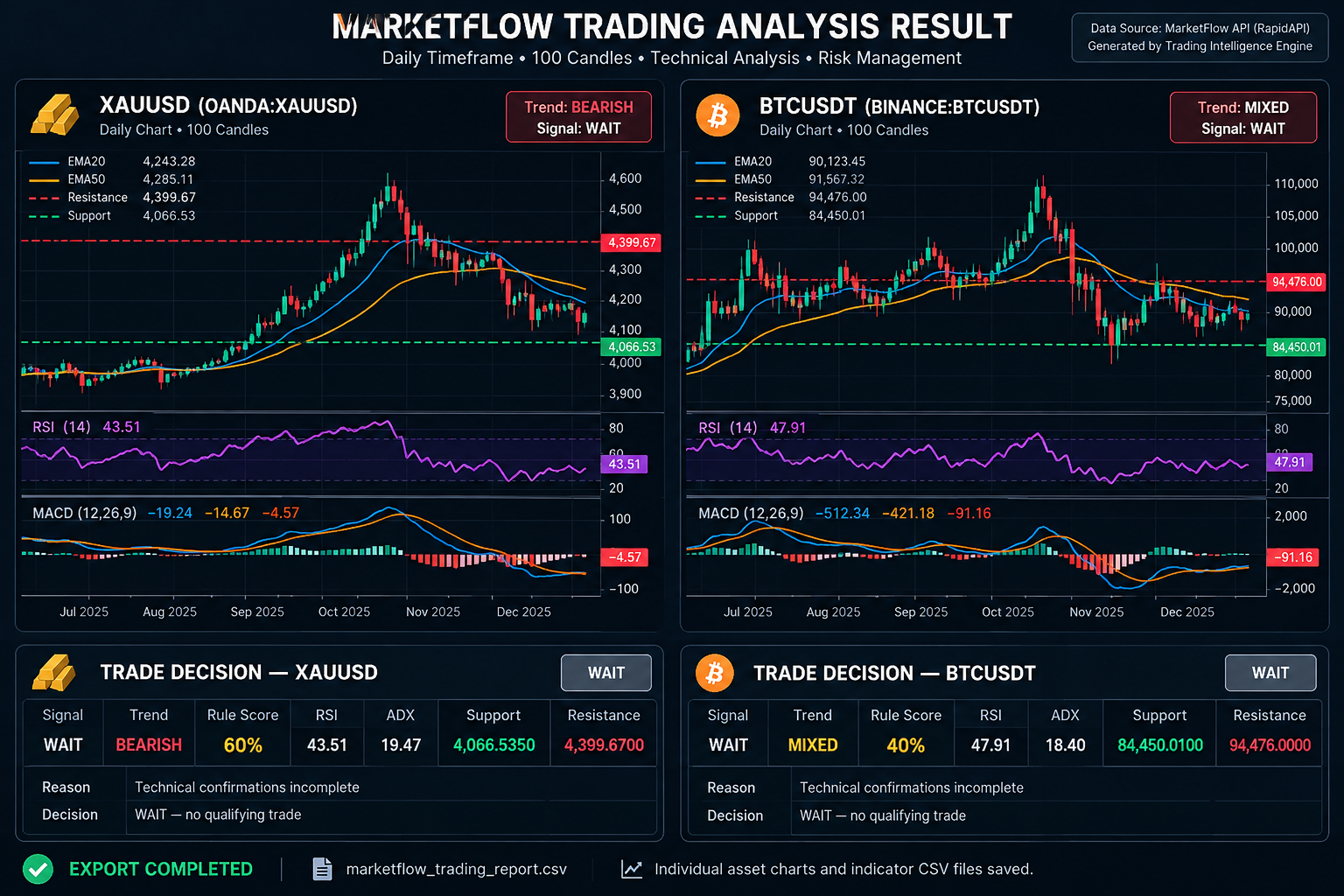
Output akhir dari Cell 5 memberikan dua jenis hasil. Pertama, sistem menghasilkan visual trading dashboard untuk setiap aset. Kedua, sistem menghasilkan decision report yang menunjukkan signal, trend, rule score, RSI, ADX, support, resistance, alasan keputusan, serta entry, stop-loss, dan target apabila setup memenuhi seluruh kondisi. marketflow_trading_intelligence
RESULT:
Conclusion
The MarketFlow Trading Intelligence Engine provides a systematic framework for analyzing XAUUSD and BTCUSDT using daily OHLCV data. The workflow begins with API configuration and market-data retrieval, followed by OHLCV normalization and validation. The normalized dataset is then processed through a technical indicator engine covering EMA20, EMA50, RSI14, MACD, ATR14, ADX14, directional indicators, support, resistance, returns, and volatility. marketflow_trading_intelligence marketflow_trading_intelligence
The signal engine requires complete alignment between five technical conditions before issuing a LONG or SHORT signal. When the confirmations are incomplete, the system returns WAIT, which prevents the model from forcing a trade under ambiguous market conditions. Risk management is integrated through ATR-based stop-loss distance, predefined reward-to-risk targets, and position sizing based on the account risk budget. marketflow_trading_intelligence
The final dashboard provides a practical representation of the analysis through candlestick charts, EMA overlays, support and resistance levels, RSI, MACD histogram, and trade levels. The system also exports the final trading report and individual indicator datasets for further quantitative analysis. marketflow_trading_intelligence
However, the output should be interpreted as a rule-based trading decision-support system, not as a guarantee of future returns. The position-sizing calculation in the source explicitly does not account for contract multipliers, transaction fees, or slippage. Therefore, the calculated quantity should be adapted to the actual instrument specifications and execution environment before live trading. marketflow_trading_intelligence
Overall, the system provides a clear research framework for transforming raw MarketFlow market data into a reproducible trading analysis process. Its main strength is the integration of multiple independent technical confirmations and explicit risk-management rules rather than relying on a single indicator or discretionary interpretation.