
Financial market analysis becomes more useful when price action is evaluated together with technical indicators and investor information. A single price series can describe market movement, but it does not provide enough context to determine trend structure, momentum, volatility, support and resistance, or the broader investment behavior associated with a market.
This project develops a MarketFlow Trader Analysis System focused on XAUUSD using daily market data and historical smart-money information associated with Warren Buffett. The system retrieves up to 100 daily XAUUSD candles from the MarketFlow API and combines them with a guru-performance dataset dated June 30, 2024. marketflow_trader_analysis
The technical analysis calculates SMA20, SMA50, RSI14, ATR14, support, and resistance. These indicators are then used to classify the current market trend and generate a conservative trading classification of WATCH LONG, WATCH SHORT, or WAIT. The system deliberately treats watch signals as setups rather than executed trades. marketflow_trader_analysis
The second analytical component examines Warren Buffett's historical portfolio information. It extracts portfolio-level metrics and attempts to identify the top holdings and their portfolio weights. This information provides additional investment context, but it is explicitly treated as historical portfolio data rather than a current XAUUSD trading signal. marketflow_trader_analysis
Cell 1 — Install Library & API Configuration
The first cell establishes the Python environment and configures the MarketFlow API. Pandas is used for data manipulation, NumPy for numerical calculations, Matplotlib and Seaborn for visualization, Requests for API communication, and JSON for handling API responses.
The system is configured for OANDA:XAUUSD on the daily timeframe with 100 requested historical candles. The smart-money dataset is configured for the investor slug warren-buffett with a report date of 2024-06-30 and the top 10 holdings. marketflow_trader_analysis
Code
%pip -q install requests pandas numpy matplotlib seaborn

import requests
import pandas as pd
import numpy as np
import matplotlib.pyplot as plt
import seaborn as sns
import json
import os
from getpass import getpass

sns.set_theme(style="darkgrid")
pd.set_option("display.max_columns", 50)

BASE_URL = "https://marketflow-all-in-one-market-finance-api.p.rapidapi.com"
API_HOST = "marketflow-all-in-one-market-finance-api.p.rapidapi.com"

API_KEY = os.getenv("RAPIDAPI_KEY") or getpass("Masukkan RapidAPI Key: ")

HEADERS = {
    "x-rapidapi-host": API_HOST,
    "x-rapidapi-key": API_KEY
}

PRICE_PARAMS = {
    "range": 100,
    "timeframe": "D",
    "timezone": "Asia/Jakarta",
    "symbol": "OANDA:XAUUSD"
}

GURU_PARAMS = {
    "report_date": "2024-06-30",
    "top_holdings": 10,
    "slug": "warren-buffett"
}

print("=" * 65)
print(" MARKETFLOW TRADER ANALYSIS")
print("=" * 65)
print("Market        : XAUUSD")
print("Timeframe     : Daily")
print("Historical    : 100 candles requested")
print("Smart Money   : Warren Buffett")
print("Guru Report   : 2024-06-30")
print("Configuration : READY")
This cell provides the control parameters for the complete analysis. The API key is requested through the environment or an interactive prompt instead of being hard-coded into the analysis. The configuration also clearly separates the XAUUSD price dataset from the historical smart-money dataset.
Cell 2 — Fetch API Data & Normalize OHLC
The second cell retrieves both datasets from MarketFlow. The /v2/chart/price endpoint provides XAUUSD price data, while /smartmoney/guru-performance provides the Warren Buffett guru-performance dataset. marketflow_trader_analysis
Because API responses may contain different structures or field names, the code searches recursively for OHLC records. It recognizes both conventional field names such as open, high, low, and close, as well as abbreviated fields such as o, h, l, and c. marketflow_trader_analysis
The timestamp is also normalized safely. The code determines whether the timestamp is expressed in seconds, milliseconds, microseconds, or nanoseconds based on its magnitude before converting it into Jakarta time. marketflow_trader_analysis
The resulting OHLC dataset is then checked for missing records, duplicate timestamps, invalid price relationships, and minimum data requirements. At least 55 candles are required because the analysis later calculates a 50-period moving average. marketflow_trader_analysis
Code
# ============================================================
# CELL 2 — MARKETFLOW API FETCH & OHLC NORMALIZATION (FIXED)
# ============================================================

import requests
import pandas as pd
import numpy as np
import json

def fetch_api(endpoint, params):
    try:
        response = requests.get(
            BASE_URL + endpoint,
            headers=HEADERS,
            params=params,
            timeout=35
        )
        response.raise_for_status()
        data = response.json()

        if isinstance(data, dict):
            if data.get("success") is False or data.get("error"):
                raise ValueError(str(data)[:500])

        print(f"[OK] {endpoint} | HTTP {response.status_code}")
        return data

    except Exception as e:
        print(f"[ERROR] {endpoint}: {e}")
        return None


# 1. FETCH BOTH ENDPOINTS
price_raw = fetch_api("/v2/chart/price", PRICE_PARAMS)
guru_raw = fetch_api("/smartmoney/guru-performance", GURU_PARAMS)


# 2. FIND OHLC RECORDS
def find_ohlc(obj, depth=0):
    if depth > 8:
        return None

    if isinstance(obj, list):
        if obj and isinstance(obj[0], dict):
            temp = pd.DataFrame(obj)
            names = set(str(c).lower() for c in temp.columns)

            if (
                {"open", "high", "low", "close"}.issubset(names)
                or {"o", "h", "l", "c"}.issubset(names)
            ):
                return temp

        for item in obj[:15]:
            result = find_ohlc(item, depth + 1)
            if result is not None:
                return result

    elif isinstance(obj, dict):
        names = set(str(k).lower() for k in obj)

        if (
            {"open", "high", "low", "close"}.issubset(names)
            or {"o", "h", "l", "c"}.issubset(names)
        ):
            if all(isinstance(v, (list, tuple)) for v in obj.values()):
                return pd.DataFrame(obj)

        for value in obj.values():
            result = find_ohlc(value, depth + 1)
            if result is not None:
                return result

    return None


df_raw = find_ohlc(price_raw)

if df_raw is None:
    print(json.dumps(price_raw, default=str)[:3000])
    raise ValueError("OHLC data not found in API response.")

print("\nRAW API COLUMNS:")
print(df_raw.columns.tolist())


# 3. SELECT COLUMNS WITHOUT DUPLICATE NAMES
def select_column(frame, candidates):
    for name in candidates:
        matching = [
            c for c in frame.columns
            if str(c).lower() == name.lower()
        ]
        if matching:
            result = frame.loc[:, matching[0]]
            if isinstance(result, pd.DataFrame):
                result = result.iloc[:, 0]
            return result.reset_index(drop=True)
    return None


df = pd.DataFrame()

column_map = {
    "open": ["open", "o"],
    "high": ["high", "h"],
    "low": ["low", "l"],
    "close": ["close", "c"],
    "volume": ["volume", "v"]
}

for target, candidates in column_map.items():
    series = select_column(df_raw, candidates)

    if series is not None:
        df[target] = pd.to_numeric(series, errors="coerce")

# Select only one timestamp field
time_series = select_column(
    df_raw,
    ["time", "timestamp", "datetime", "date", "t"]
)

if time_series is None:
    raise ValueError("Timestamp column not found.")


# 4. CONVERT TIMESTAMP SAFELY
numeric_time = pd.to_numeric(time_series, errors="coerce")

if numeric_time.notna().all():
    magnitude = numeric_time.abs().median()

    if magnitude > 1e17:
        unit = "ns"
    elif magnitude > 1e14:
        unit = "us"
    elif magnitude > 1e11:
        unit = "ms"
    else:
        unit = "s"

    parsed_time = pd.to_datetime(
        numeric_time, unit=unit,
        utc=True, errors="coerce"
    )

else:
    parsed_time = pd.to_datetime(
        time_series,
        utc=True,
        errors="coerce"
    )

df["time"] = parsed_time.dt.tz_convert("Asia/Jakarta")


# 5. CLEAN DATA
required = ["time", "open", "high", "low", "close"]

df = (
    df.dropna(subset=required)
      .sort_values("time")
      .drop_duplicates(subset=["time"])
      .reset_index(drop=True)
)

if df.empty:
    raise ValueError("No valid OHLC records after normalization.")

valid_ohlc = (
    (df["high"] >= df[["open", "close", "low"]].max(axis=1))
    & (df["low"] <= df[["open", "close", "high"]].min(axis=1))
    & (df["low"] > 0)
)

invalid_count = int((~valid_ohlc).sum())

if invalid_count:
    raise ValueError(
        f"{invalid_count} invalid OHLC records detected."
    )

if len(df) < 55:
    raise ValueError(
        f"Insufficient candles: {len(df)}. Minimum 55 required."
    )


# 6. OUTPUT
print("\n" + "=" * 65)
print(" XAUUSD DATA VALIDATION")
print("=" * 65)

print("Status          : SUCCESS")
print("Total Candles   :", len(df))
print("First Candle    :", df["time"].iloc[0])
print("Last Candle     :", df["time"].iloc[-1])
print("Latest Close    :", round(float(df["close"].iloc[-1]), 3))
print("Duplicate Time  :", df["time"].duplicated().sum())
print("Invalid OHLC    :", invalid_count)
print("Guru API        :", "AVAILABLE" if guru_raw is not None else "UNAVAILABLE")

print("\nLATEST 10 CANDLES")
display(df.tail(10))

print("\nCELL 2 COMPLETED — READY FOR CELL 3")
The main purpose of this cell is to ensure that the technical analysis is performed on a clean and structurally valid OHLC dataset rather than directly on an unprocessed API response.
Cell 3 — Technical Analysis & Trading Signal
Cell 3 calculates the main technical indicators used by the trading engine.
The system calculates SMA20 and SMA50 to represent short- and medium-term price structure. RSI14 is calculated using Wilder-style exponential smoothing, while ATR14 measures the current price range and volatility. Support and resistance are derived from the previous 20 candles using .shift(1), which avoids incorporating the current candle into its own reference levels. marketflow_trader_analysis
The trend classification follows three conditions:
Price > SMA20 > SMA50 → BULLISH
Price < SMA20 < SMA50 → BEARISH
Otherwise              → SIDEWAYS / MIXED
The signal engine is intentionally conservative. A bullish market only produces WATCH LONG when RSI is between 50 and 70. A bearish market only produces WATCH SHORT when RSI is between 30 and 50. Otherwise, the system remains at WAIT. marketflow_trader_analysis
The stop-loss is positioned at 1.5 ATR from the entry and the take-profit at 3 ATR. Therefore, the setup has a nominal reward-to-risk ratio of:
\[ RR = \frac{3ATR}{1.5ATR} = 2.0 \]
The source code calculates this explicitly before generating the final analysis dictionary. marketflow_trader_analysis
Code
# CELL 3 — XAUUSD TECHNICAL ANALYSIS

# Moving averages
df["SMA20"] = df["close"].rolling(20).mean()
df["SMA50"] = df["close"].rolling(50).mean()

# RSI Wilder (14)
delta = df["close"].diff()
gain = delta.clip(lower=0)
loss = -delta.clip(upper=0)

avg_gain = gain.ewm(
    alpha=1/14, adjust=False, min_periods=14
).mean()

avg_loss = loss.ewm(
    alpha=1/14, adjust=False, min_periods=14
).mean()

rs = avg_gain / avg_loss.replace(0, np.nan)
df["RSI14"] = 100 - (100 / (1 + rs))
df.loc[(avg_loss == 0) & (avg_gain > 0), "RSI14"] = 100
df.loc[(avg_gain == 0) & (avg_loss > 0), "RSI14"] = 0
df.loc[(avg_gain == 0) & (avg_loss == 0), "RSI14"] = 50

# Average True Range
previous_close = df["close"].shift(1)

tr = pd.concat([
    df["high"] - df["low"],
    (df["high"] - previous_close).abs(),
    (df["low"] - previous_close).abs()
], axis=1).max(axis=1)

df["ATR14"] = tr.ewm(
    alpha=1/14, adjust=False, min_periods=14
).mean()

# Prior support/resistance: no look-ahead
df["Support"] = df["low"].shift(1).rolling(20).min()
df["Resistance"] = df["high"].shift(1).rolling(20).max()

# Latest indicators
last = df.iloc[-1]

price = float(last["close"])
sma20 = float(last["SMA20"])
sma50 = float(last["SMA50"])
rsi = float(last["RSI14"])
atr = float(last["ATR14"])
support = float(last["Support"])
resistance = float(last["Resistance"])

# Trend classification
if price > sma20 > sma50:
    trend = "BULLISH"
elif price < sma20 < sma50:
    trend = "BEARISH"
else:
    trend = "SIDEWAYS / MIXED"

# Conservative signal classification
signal = "WAIT"
entry = stop_loss = take_profit = np.nan
reason = "Belum ada konfirmasi tren dan momentum."

if trend == "BULLISH" and 50 < rsi < 70:
    signal = "WATCH LONG"
    entry = price
    stop_loss = entry - 1.5 * atr
    take_profit = entry + 3.0 * atr
    reason = "Bullish MA alignment and positive RSI."

elif trend == "BEARISH" and 30 < rsi < 50:
    signal = "WATCH SHORT"
    entry = price
    stop_loss = entry + 1.5 * atr
    take_profit = entry - 3.0 * atr
    reason = "Bearish MA alignment and negative RSI."

risk = abs(entry - stop_loss) if np.isfinite(entry) else np.nan
reward = abs(take_profit - entry) if np.isfinite(entry) else np.nan
rr = reward / risk if np.isfinite(risk) and risk > 0 else np.nan

analysis = {
    "Symbol": "OANDA:XAUUSD",
    "Timeframe": "D",
    "Last Candle": str(last["time"]),
    "Price": round(price, 3),
    "SMA20": round(sma20, 3),
    "SMA50": round(sma50, 3),
    "RSI14": round(rsi, 2),
    "ATR14": round(atr, 3),
    "Support": round(support, 3),
    "Resistance": round(resistance, 3),
    "Trend": trend,
    "Signal": signal,
    "Entry Reference": round(entry, 3) if np.isfinite(entry) else None,
    "Stop Loss": round(stop_loss, 3) if np.isfinite(stop_loss) else None,
    "Take Profit": round(take_profit, 3) if np.isfinite(take_profit) else None,
    "Risk Reward": round(rr, 2) if np.isfinite(rr) else None,
    "Reason": reason
}

print("=" * 60)
print("XAUUSD TECHNICAL TRADING ANALYSIS")
print("=" * 60)

for key, value in analysis.items():
    print(f"{key:<20}: {value}")

print("\nNOTE: WATCH signals are setups, not executed trades.")
This cell converts the raw market data into a structured trading interpretation. Importantly, the signal is not generated simply because the market is bullish or bearish. RSI must also satisfy the defined momentum range.
Cell 4 — Warren Buffett Smart Money & Guru Performance
The fourth cell analyzes the historical guru-performance response.
The raw response is saved as guru_performance_raw.json for auditability. The code then recursively flattens scalar metrics and searches for holding-related arrays using keywords such as holding, position, or stock. marketflow_trader_analysis
When holdings are available, the system selects the top 10 records and attempts to identify the portfolio-weight field and company or ticker field automatically. If portfolio weights are expressed as fractions between 0 and 1, they are converted into percentages. The sum of the top holdings' weights is then reported and visualized. marketflow_trader_analysis
The critical limitation is already recognized in the source code: this is historical portfolio information, not a current XAUUSD signal. marketflow_trader_analysis
Code
# CELL 4 — GURU PERFORMANCE ANALYSIS

print("=" * 65)
print("WARREN BUFFETT — SMART MONEY ANALYSIS")
print("=" * 65)

if guru_raw is None:
    guru_data = {}
    print("Guru API unavailable.")
else:
    guru_data = guru_raw

# Save raw response for audit
with open("guru_performance_raw.json", "w", encoding="utf-8") as f:
    json.dump(guru_data, f, indent=2, default=str)

def flatten_scalars(obj, prefix="", depth=0):
    result = {}
    if not isinstance(obj, dict) or depth > 4:
        return result

    for key, value in obj.items():
        path = f"{prefix}.{key}" if prefix else key

        if isinstance(value, dict):
            result.update(flatten_scalars(value, path, depth + 1))
        elif isinstance(value, (str, int, float, bool)):
            result[path] = value

    return result


def find_holdings(obj, depth=0):
    if depth > 7:
        return None

    if isinstance(obj, dict):
        for key, value in obj.items():
            if (
                isinstance(value, list)
                and len(value) > 0
                and isinstance(value[0], dict)
                and any(
                    word in key.lower()
                    for word in ["holding", "position", "stock"]
                )
            ):
                return pd.DataFrame(value)

        for value in obj.values():
            result = find_holdings(value, depth + 1)
            if result is not None:
                return result

    elif isinstance(obj, list):
        for item in obj[:10]:
            result = find_holdings(item, depth + 1)
            if result is not None:
                return result

    return None


# Portfolio metrics
metrics = flatten_scalars(guru_data)

print("\nPORTFOLIO PERFORMANCE METRICS")
for key, value in metrics.items():
    print(f"{key:<45}: {value}")

# Top holdings
holdings = find_holdings(guru_data)

if holdings is not None and not holdings.empty:
    holdings = holdings.head(10).copy()

    print("\nTOP 10 HOLDINGS")
    display(holdings)

    # Detect portfolio weight column
    weight_candidates = [
        c for c in holdings.columns
        if any(k in c.lower() for k in [
            "weight", "portfolio_pct",
            "allocation", "percent"
        ])
    ]

    name_candidates = [
        c for c in holdings.columns
        if c.lower() in [
            "ticker", "symbol", "stock",
            "company", "name", "t"
        ]
    ]

    if weight_candidates and name_candidates:
        weight_col = weight_candidates[0]
        name_col = name_candidates[0]

        weights = pd.to_numeric(
            holdings[weight_col].astype(str).str.replace(
                "%", "", regex=False
            ),
            errors="coerce"
        )

        # Convert fractional weights to percentages
        if weights.notna().any() and weights.max() <= 1:
            weights = weights * 100

        holdings["weight_pct"] = weights

        top_concentration = weights.sum()

        print(f"\nTop Holdings Weight Sum: {top_concentration:.2f}%")

        fig, ax = plt.subplots(figsize=(11, 5))
        ax.barh(
            holdings[name_col].astype(str),
            holdings["weight_pct"],
            color="#27ae60"
        )
        ax.invert_yaxis()
        ax.set_title("Warren Buffett — Top Portfolio Holdings")
        ax.set_xlabel("Portfolio Weight (%)")
        plt.tight_layout()
        plt.show()

    else:
        print("Holding weights are not available in the response.")

else:
    print("\nTop holdings not found in API response.")

print("\nReport requested: 2024-06-30")
print("Historical portfolio data, not a current gold trading signal.")
The purpose of this cell is not to claim that Warren Buffett's historical holdings predict XAUUSD. Instead, it provides a separate smart-money information layer that can be reviewed alongside the technical analysis.
Cell 5 — Professional Trading Dashboard & Export
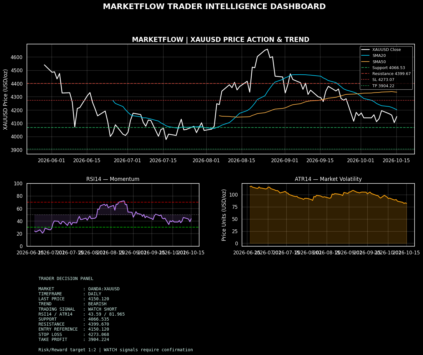
The final cell consolidates the technical analysis into a professional dashboard.
The dashboard contains four major components:
XAUUSD Price Action & Trend
RSI14 Momentum
ATR14 Market Volatility
Trader Decision Panel
The first chart plots XAUUSD closing price against SMA20 and SMA50 and adds the calculated support and resistance levels. If a trading setup exists, stop-loss and take-profit levels are also displayed. marketflow_trader_analysis
The second chart visualizes RSI14 with 30, 50, and 70 reference levels. The third chart displays ATR14 as a volatility measure. The final panel summarizes the market, timeframe, price, trend, trading signal, RSI, ATR, support, resistance, entry reference, stop-loss, and take-profit. marketflow_trader_analysis
The system finally exports:
trader_dashboard_xauusd.png
xauusd_indicators.csv
guru_performance_raw.json
trader_signal_summary.json
These outputs are explicitly generated by the source code. marketflow_trader_analysis
Code
# CELL 5 — TRADING DASHBOARD & EXPORT

from matplotlib.gridspec import GridSpec

plt.style.use("dark_background")

fig = plt.figure(figsize=(16, 12))
gs = GridSpec(
    3, 2, figure=fig,
    height_ratios=[2.1, 1.2, 1.1],
    hspace=0.38, wspace=0.25
)

# 1. Price and moving averages
ax1 = fig.add_subplot(gs[0, :])

ax1.plot(
    df["time"], df["close"],
    label="XAUUSD Close", color="white", linewidth=1.9
)
ax1.plot(
    df["time"], df["SMA20"],
    label="SMA20", color="#00d4ff", linewidth=1.4
)
ax1.plot(
    df["time"], df["SMA50"],
    label="SMA50", color="#ffb347", linewidth=1.4
)

ax1.axhline(
    support, color="#2ecc71",
    linestyle="--", alpha=0.8,
    label=f"Support {support:.2f}"
)
ax1.axhline(
    resistance, color="#e74c3c",
    linestyle="--", alpha=0.8,
    label=f"Resistance {resistance:.2f}"
)

if np.isfinite(entry):
    ax1.axhline(
        stop_loss, color="#ff4d4d",
        linestyle=":", label=f"SL {stop_loss:.2f}"
    )
    ax1.axhline(
        take_profit, color="#2ecc71",
        linestyle=":", label=f"TP {take_profit:.2f}"
    )

ax1.set_title(
    "MARKETFLOW | XAUUSD PRICE ACTION & TREND",
    fontsize=15, fontweight="bold"
)
ax1.set_ylabel("XAUUSD Price (USD/oz)")
ax1.legend(loc="best", fontsize=9)
ax1.grid(alpha=0.2)

# 2. RSI chart
ax2 = fig.add_subplot(gs[1, 0])
ax2.plot(
    df["time"], df["RSI14"],
    color="#c084fc", linewidth=1.8
)
ax2.axhline(70, color="red", linestyle="--", alpha=0.7)
ax2.axhline(30, color="lime", linestyle="--", alpha=0.7)
ax2.axhline(50, color="gray", linestyle=":", alpha=0.7)
ax2.fill_between(
    df["time"], df["RSI14"], 50,
    alpha=0.12, color="#c084fc"
)
ax2.set_ylim(0, 100)
ax2.set_title("RSI14 — Momentum")
ax2.grid(alpha=0.2)

# 3. ATR chart
ax3 = fig.add_subplot(gs[1, 1])
ax3.plot(
    df["time"], df["ATR14"],
    color="#f59e0b", linewidth=1.8
)
ax3.fill_between(
    df["time"], df["ATR14"],
    alpha=0.2, color="#f59e0b"
)
ax3.set_title("ATR14 — Market Volatility")
ax3.set_ylabel("Price Units (USD/oz)")
ax3.grid(alpha=0.2)

# 4. Trading summary
ax4 = fig.add_subplot(gs[2, :])
ax4.axis("off")

summary_lines = [
    "TRADER DECISION PANEL",
    "",
    f"MARKET           : OANDA:XAUUSD",
    f"TIMEFRAME        : DAILY",
    f"LAST PRICE       : {price:.3f}",
    f"TREND            : {trend}",
    f"TRADING SIGNAL   : {signal}",
    f"RSI14 / ATR14    : {rsi:.2f} / {atr:.3f}",
    f"SUPPORT          : {support:.3f}",
    f"RESISTANCE       : {resistance:.3f}",
    f"ENTRY REFERENCE  : {entry:.3f}" if np.isfinite(entry) else "ENTRY REFERENCE  : N/A",
    f"STOP LOSS        : {stop_loss:.3f}" if np.isfinite(stop_loss) else "STOP LOSS        : N/A",
    f"TAKE PROFIT      : {take_profit:.3f}" if np.isfinite(take_profit) else "TAKE PROFIT      : N/A",
    "",
    "Risk/Reward target 1:2 | WATCH signals require confirmation"
]

ax4.text(
    0.03, 0.98,
    "\n".join(summary_lines),
    va="top", ha="left",
    fontfamily="monospace",
    fontsize=10, color="#d7f9f1",
    transform=ax4.transAxes
)

fig.suptitle(
    "MARKETFLOW TRADER INTELLIGENCE DASHBOARD",
    fontsize=18, fontweight="bold", y=0.99
)

plt.savefig(
    "trader_dashboard_xauusd.png",
    dpi=220, bbox_inches="tight"
)
plt.show()

# Export technical data
df.to_csv("xauusd_indicators.csv", index=False)

# Export decision
with open("trader_signal_summary.json", "w") as f:
    json.dump(analysis, f, indent=2)

print("\n" + "=" * 65)
print("ANALYSIS COMPLETE")
print("=" * 65)

print("1. trader_dashboard_xauusd.png")
print("2. xauusd_indicators.csv")
print("3. guru_performance_raw.json")
print("4. trader_signal_summary.json")
print("\nTrading dashboard successfully generated.")
The dashboard therefore functions as the final presentation layer of the system. Instead of displaying only a numerical signal, it combines price structure, moving averages, momentum, volatility, support/resistance, and the current decision into a single research dashboard.
RESULT:
Conclusion
The MarketFlow Trader Analysis System provides a structured workflow for evaluating XAUUSD through technical market data and historical smart-money information. The system begins with API configuration, retrieves XAUUSD daily data, normalizes the API response, validates the OHLC structure, and calculates the technical indicators required for the trading decision.
The technical engine uses SMA20, SMA50, RSI14, ATR14, support, and resistance to classify the current market structure. A bullish structure with RSI between 50 and 70 generates a WATCH LONG setup, while a bearish structure with RSI between 30 and 50 generates a WATCH SHORT setup. All other conditions remain classified as WAIT. marketflow_trader_analysis
Risk management is integrated through an ATR-based stop-loss and take-profit framework. The source uses 1.5 ATR for the stop-loss and 3 ATR for the take-profit, producing a nominal 2:1 reward-to-risk ratio when a setup exists. marketflow_trader_analysis
The smart-money component adds historical portfolio context through Warren Buffett's June 30, 2024 guru-performance report. However, this information must not be interpreted as a current XAUUSD trading signal. The source itself explicitly identifies the guru data as historical portfolio information. marketflow_trader_analysis
Finally, the system produces a visual XAUUSD trading dashboard and exports the technical dataset, raw guru response, and trading decision summary. This creates a reproducible workflow from raw API data to structured technical analysis and research output. marketflow_trader_analysis
Overall, the system should be treated as a trading research and decision-support framework, not an automatic trading strategy. The WATCH LONG and WATCH SHORT classifications represent potential setups that still require confirmation from price action, market context, execution conditions, and appropriate risk management.