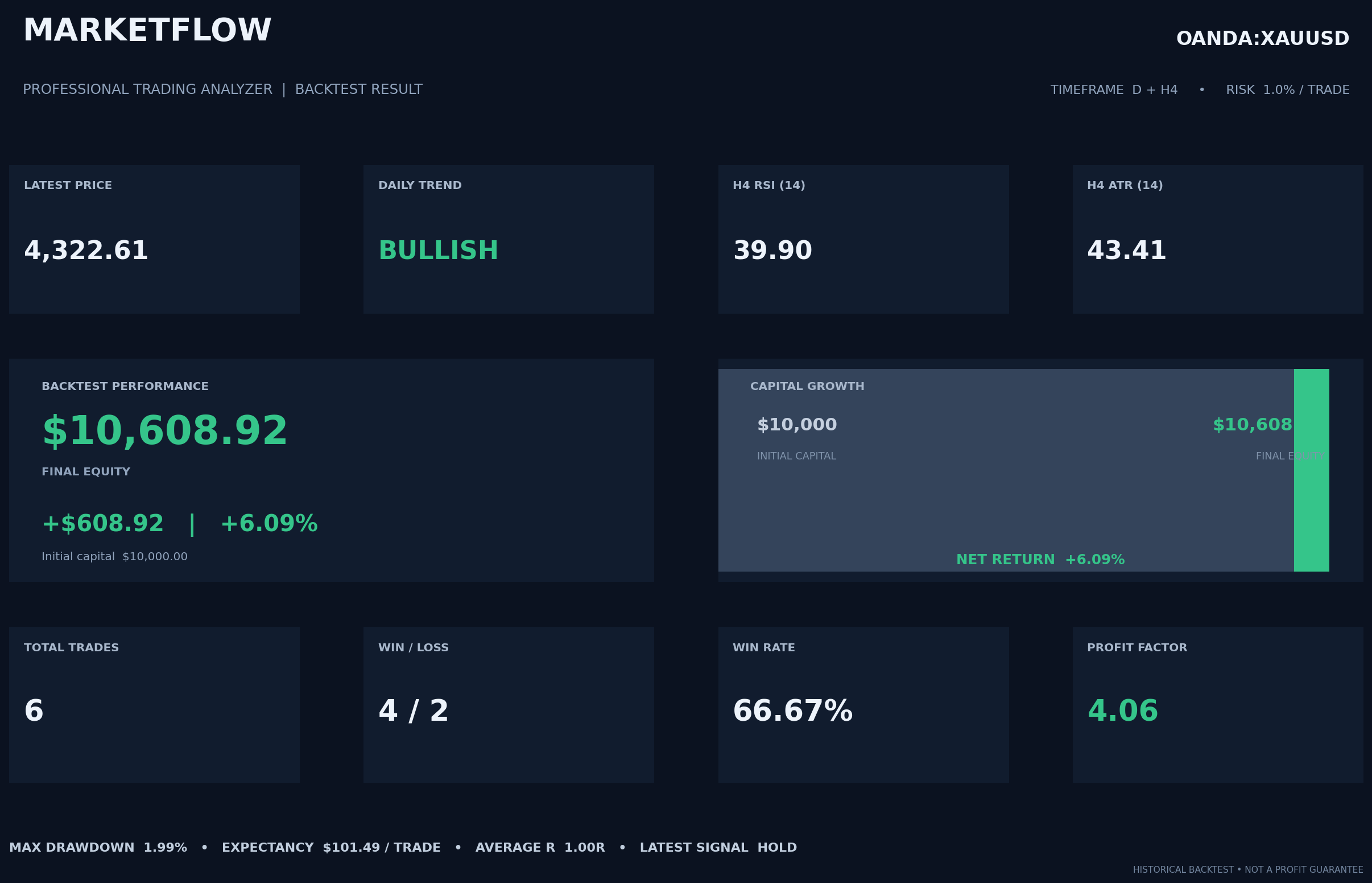
This article presents MarketFlow Professional Trading Analyzer, a Python-based framework for analyzing XAUUSD through a multi-timeframe trend-following strategy. The system retrieves Daily and four-hour (H4) market candles from the MarketFlow All-in-One Market Finance API, processes OHLC data, calculates EMA20, EMA50, RSI14, MACD, and ATR14, and combines higher-timeframe trend direction with H4 entry conditions. It further implements ATR-based stop-loss and take-profit levels, risk-based position sizing, historical backtesting, performance statistics, visualizations, and CSV exports. The supplied source code covers the full analytical workflow. Since no execution log or verified backtest output accompanies the source file, this article describes the framework and its generated evaluation measures without claiming specific profitability results.
1. Introduction
The financial market is characterized by continuous price fluctuations influenced by economic conditions, monetary policies, geopolitical developments, and investor behavior. Gold (XAUUSD) is one of the actively traded financial instruments because of its role as a safe-haven asset and its sensitivity to global economic uncertainty. Analyzing gold price movements therefore requires a systematic approach that can identify market trends, evaluate trading opportunities, and manage potential risks.
Technical analysis provides tools for examining historical price movements and identifying potential market directions. Indicators such as the Exponential Moving Average (EMA), Relative Strength Index (RSI), Moving Average Convergence Divergence (MACD), and Average True Range (ATR) are used in this framework to evaluate trend, momentum, and volatility.
However, relying on a single timeframe may produce signals that conflict with the broader market direction. A short-term bullish movement, for example, may occur within a broader bearish trend. A multi-timeframe approach can reduce this fragmentation by using a higher timeframe to define market direction and a lower timeframe to identify potential entries.
This article presents MarketFlow Professional Trading Analyzer, a Python-based framework that integrates Daily and four-hour (H4) market data obtained through the MarketFlow All-in-One Market Finance API. The system applies a trend-following strategy to the OANDA:XAUUSD instrument. The Daily timeframe is used to determine the broader trend, while the H4 timeframe is used to identify entry opportunities through EMA structure, price crossover, RSI, and MACD confirmation.
The framework also includes ATR-based stop-loss and take-profit calculations, position sizing based on a predefined risk percentage, historical backtesting, performance evaluation, chart generation, and CSV data export. Its objective is to provide a reproducible workflow that connects market data retrieval, technical analysis, trading simulation, and reporting in one Python program.
2. Methodology
2.1. System Configuration and Market Data Source
The system uses Python libraries including Requests, NumPy, Pandas, and Matplotlib. Requests handles communication with the MarketFlow API, Pandas organizes and processes the candle data, NumPy supports numerical calculations, and Matplotlib generates visual outputs.
The instrument is configured as OANDA:XAUUSD, with the query symbol XAUUSD and the Asia/Jakarta timezone. The historical period specified in the source code is 1 January 2025 to 31 December 2025. Two timeframes are retrieved: Daily (D) and four-hour (H4), represented by the API timeframe values D and 240.
The API request function includes a retry mechanism for timeout and connection errors. It also checks HTTP response status and returns JSON data for subsequent processing. API credentials should be supplied through an environment variable rather than embedded directly in a published source file.
Code — Cell 1: Configuration and API
# -*- coding: utf-8 -*-
"""marketflow_professional_analyzer.ipynb

Automatically generated by Colab.

Original file is located at
    https://colab.research.google.com/drive/1YivxBwsjFWmXmDHumlxB0aKhoNAcGQQ1

CELL 1 — Configuration & API
"""

# ==========================================================
# CELL 1 — MARKETFLOW PROFESSIONAL TRADING ANALYZER
# ==========================================================

import os
import json
import time
import requests
import numpy as np
import pandas as pd
import matplotlib.pyplot as plt
import matplotlib.dates as mdates

from matplotlib.patches import Rectangle
from datetime import datetime

# ==========================================================
# RAPIDAPI CONFIGURATION
# ==========================================================

API_KEY = os.getenv("RAPIDAPI_KEY", "MASUKKAN_RAPIDAPI_KEY_KAMU")

API_HOST = "marketflow-all-in-one-market-finance-api.p.rapidapi.com"

BASE_URL = f"https://{API_HOST}"

HEADERS = {
    "x-rapidapi-key": API_KEY,
    "x-rapidapi-host": API_HOST
}

if not API_KEY or API_KEY == "MASUKKAN_RAPIDAPI_KEY_KAMU":
    raise ValueError("RapidAPI Key belum dimasukkan.")

# ==========================================================
# MARKET CONFIGURATION
# ==========================================================

SYMBOL = "OANDA:XAUUSD"

QUERY = "XAUUSD"

TIMEZONE = "Asia/Jakarta"

TIMEFRAMES = {
    "D": "D",
    "H4": "240"
}

DATE_FROM = "2025-01-01"
DATE_TO = "2025-12-31"

# ==========================================================
# STRATEGY CONFIGURATION
# ==========================================================

INITIAL_CAPITAL = 10000.0

RISK_PERCENT = 1.0

ATR_SL_MULTIPLIER = 1.5

ATR_TP_MULTIPLIER = 3.0

EMA_FAST = 20

EMA_SLOW = 50

RSI_PERIOD = 14

ATR_PERIOD = 14

# Biaya transaksi dalam satuan harga per unit.
# Isi sesuai spesifikasi broker jika diketahui.
SLIPPAGE_PRICE = 0.0

COMMISSION_PER_UNIT = 0.0

# ==========================================================
# OUTPUT
# ==========================================================

OUTPUT_DIR = "marketflow_professional"

os.makedirs(OUTPUT_DIR, exist_ok=True)

# ==========================================================
# API REQUEST WITH RETRY
# ==========================================================

def marketflow_get(endpoint, params=None, retries=3):

    url = BASE_URL + endpoint

    for attempt in range(1, retries + 1):

        try:

            print(
                f"REQUEST {endpoint} "
                f"| Attempt {attempt}/{retries}"
            )

            response = requests.get(
                url,
                headers=HEADERS,
                params=params,
                timeout=(20, 120)
            )

            response.raise_for_status()

            print("STATUS:", response.status_code)

            return response.json()

        except requests.exceptions.Timeout:

            print("API TIMEOUT")

        except requests.exceptions.ConnectionError:

            print("CONNECTION ERROR")

        except requests.exceptions.HTTPError:

            print("HTTP ERROR:", response.status_code)

            print(response.text[:1000])

            raise

        if attempt < retries:

            wait = attempt * 5

            print(f"Retry in {wait} seconds")

            time.sleep(wait)

    raise TimeoutError(
        f"API failed: {endpoint}"
    )


# ==========================================================
# STATUS
# ==========================================================

print("=" * 55)

print("MARKETFLOW PROFESSIONAL TRADING ANALYZER")

print("=" * 55)

print("Symbol:", SYMBOL)

print("Timeframes:", list(TIMEFRAMES.keys()))

print("Strategy: TREND FOLLOWING")

print("Risk:", RISK_PERCENT, "%")

print("Initial Capital:", INITIAL_CAPITAL)

print("Historical Period:", DATE_FROM, "-", DATE_TO)

print("=" * 55)

# ==========================================================
# DIAGNOSTIC — MARKETFLOW TIMEFRAME DOCUMENTATION
# ==========================================================

print("FETCHING MARKETFLOW API GUIDE...")

guide = marketflow_get(
    "/v2/how-to-use"
)

print("\n========== API GUIDE ==========")

print(json.dumps(
    guide,
    indent=2,
    ensure_ascii=False
)[:12000])

print("\n========== END GUIDE ==========")
2.2. Multi-Timeframe Market Data Collection
The second stage searches for the XAUUSD instrument and retrieves historical candles for both Daily and H4 timeframes. Each request includes the configured timezone, timeframe, date range, and symbol.
The returned data are checked for a successful API response and for the presence of candle records. The program stores the raw responses in a dictionary indexed by timeframe. This structure allows the subsequent processing stage to handle Daily and H4 data independently before combining their analytical features.
Code — Cell 2: Market Search and Multi-Timeframe Data
"""CELL 2 — Market Search & Multi-Timeframe Data"""

# ==========================================================
# CELL 2 — DAILY + H4 DATA COLLECTION
# ==========================================================

# MARKET SEARCH

search_result = marketflow_get(
    "/v2/search/market",
    {"query": QUERY}
)

print("MARKET SEARCH SUCCESS")

# ==========================================================
# FETCH DAILY AND H4
# ==========================================================

raw_data = {}

for tf, api_tf in TIMEFRAMES.items():

    print("\nFETCHING:", tf)

    params = {

        "timezone": TIMEZONE,

        "timeframe": api_tf,

        "from": DATE_FROM,

        "to": DATE_TO,

        "symbol": SYMBOL

    }

    result = marketflow_get(
        "/v2/chart/range",
        params
    )

    if not result.get("success"):

        raise ValueError(
            f"API failed for {tf}"
        )

    data = result.get("data", [])

    if not data:

        raise ValueError(
            f"No data received for {tf}"
        )

    raw_data[tf] = result

    print(
        tf,
        "CANDLES:",
        len(data)
    )

# ==========================================================
# VALIDATION
# ==========================================================

print("\nMULTI-TIMEFRAME VALIDATION")

for tf, payload in raw_data.items():

    print(
        tf,
        "|",
        len(payload["data"]),
        "candles"
    )

print("\nDAILY + H4 DATA READY")

display(
    pd.DataFrame(
        raw_data["H4"]["data"]
    ).head()
)
2.3. Data Normalization and Technical Indicators
The data-processing stage extracts candle rows from the API response and normalizes the field names into a consistent OHLCV structure: time, open, high, low, close, and volume. It supports alternative field names such as timestamp, datetime, o, h, l, and c.
Timestamp values are converted into the Asia/Jakarta timezone. Numeric fields are converted to numeric data types, invalid rows are removed, duplicate timestamps are eliminated, and basic price validation is applied. The program requires at least 60 candles for each timeframe.
Five technical indicator outputs are then calculated:
EMA20 and EMA50: Exponential moving averages used to describe short- and longer-period price trends.
RSI14: A momentum indicator calculated using exponentially smoothed gains and losses.
MACD: The difference between 12-period and 26-period exponential moving averages, accompanied by a 9-period signal line and histogram.
ATR14: Average True Range calculated from the maximum of the current high-low range and the two previous-close gap measures.
The code assigns an available_at timestamp to each candle. Daily candles are treated as available 24 hours after their timestamp, while H4 candles are treated as available four hours after their timestamp. The Daily features are then merged into the H4 dataset using an as-of merge. This is intended to ensure that the H4 analysis uses the latest Daily information considered available at that point in the simulation.
The higher-timeframe trend is classified as bullish when the Daily close is above its EMA50 and bearish when it is below its EMA50. On H4, bullish structure requires the close to be above EMA20 and EMA20 to be above EMA50. Bearish structure applies the inverse relationship.
Code — Cell 3: Data Processing, Indicators, and Trend Detection
"""CELL 3 — Data Processing, Indicators & Trend Detection"""

# ==========================================================
# CELL 3 — DATA PROCESSING & DAILY + H4 ANALYSIS
# ==========================================================

# ==========================================================
# 1. EXTRACT MARKETFLOW DATA
# ==========================================================

def extract_rows(payload):

    if isinstance(payload, dict):

        if not payload.get("success", False):

            raise ValueError(
                "Marketflow API response unsuccessful."
            )

        rows = payload.get("data", [])

        if isinstance(rows, list):
            return rows

    elif isinstance(payload, list):

        return payload

    return []


# ==========================================================
# 2. NORMALIZE OHLCV
# ==========================================================

def normalize_data(payload, timeframe):

    rows = extract_rows(payload)

    if not rows:

        raise ValueError(
            f"No candle data detected for {timeframe}"
        )

    data = pd.DataFrame(rows)

    aliases = {
        "time": ["time", "timestamp", "datetime", "date", "t"],
        "open": ["open", "o"],
        "high": ["high", "h"],
        "low": ["low", "l"],
        "close": ["close", "c"],
        "volume": ["volume", "vol", "v"]
    }

    lower_map = {
        str(k).lower(): k
        for k in data.columns
    }

    rename = {}

    for target, options in aliases.items():

        for option in options:

            if option in lower_map:

                rename[lower_map[option]] = target

                break

    data.rename(columns=rename, inplace=True)

    required = [
        "time",
        "open",
        "high",
        "low",
        "close"
    ]

    missing = [
        col for col in required
        if col not in data.columns
    ]

    if missing:

        raise ValueError(
            f"{timeframe}: Missing columns {missing}"
        )

    if "volume" not in data.columns:

        data["volume"] = np.nan

    # Timestamp conversion
    if pd.api.types.is_numeric_dtype(data["time"]):

        median_time = data["time"].dropna().median()

        unit = "ms" if median_time > 10**11 else "s"

        data["time"] = pd.to_datetime(
            data["time"],
            unit=unit,
            utc=True
        ).dt.tz_convert(TIMEZONE)

    else:

        data["time"] = pd.to_datetime(
            data["time"],
            errors="coerce"
        )

        if data["time"].dt.tz is None:

            data["time"] = data["time"].dt.tz_localize(
                TIMEZONE,
                nonexistent="shift_forward",
                ambiguous="NaT"
            )

        else:

            data["time"] = data["time"].dt.tz_convert(
                TIMEZONE
            )

    # Numeric conversion
    for col in [
        "open",
        "high",
        "low",
        "close",
        "volume"
    ]:

        data[col] = pd.to_numeric(
            data[col],
            errors="coerce"
        )

    data = (
        data.dropna(subset=required)
            .sort_values("time")
            .drop_duplicates("time")
            .reset_index(drop=True)
    )

    # Price validation
    data = data[
        (data["open"] > 0) &
        (data["high"] > 0) &
        (data["low"] > 0) &
        (data["close"] > 0) &
        (data["high"] >= data["low"])
    ].copy()

    data.reset_index(drop=True, inplace=True)

    if len(data) < 60:

        raise ValueError(
            f"{timeframe}: Minimum 60 candles required."
        )

    return data


# ==========================================================
# 3. CALCULATE TECHNICAL INDICATORS
# ==========================================================

def calculate_indicators(data):

    data = data.copy()

    # EMA 20
    data["EMA20"] = data["close"].ewm(
        span=20,
        adjust=False
    ).mean()

    # EMA 50
    data["EMA50"] = data["close"].ewm(
        span=50,
        adjust=False
    ).mean()

    # RSI 14
    delta = data["close"].diff()

    gain = delta.clip(lower=0)

    loss = -delta.clip(upper=0)

    avg_gain = gain.ewm(
        alpha=1/14,
        min_periods=14,
        adjust=False
    ).mean()

    avg_loss = loss.ewm(
        alpha=1/14,
        min_periods=14,
        adjust=False
    ).mean()

    rs = avg_gain / avg_loss.replace(0, np.nan)

    data["RSI14"] = 100 - (
        100 / (1 + rs)
    )

    data.loc[
        (avg_loss == 0) & (avg_gain > 0),
        "RSI14"
    ] = 100

    data.loc[
        (avg_loss == 0) & (avg_gain == 0),
        "RSI14"
    ] = 50

    # MACD
    ema12 = data["close"].ewm(
        span=12,
        adjust=False
    ).mean()

    ema26 = data["close"].ewm(
        span=26,
        adjust=False
    ).mean()

    data["MACD"] = ema12 - ema26

    data["MACD_SIGNAL"] = data["MACD"].ewm(
        span=9,
        adjust=False
    ).mean()

    data["MACD_HIST"] = (
        data["MACD"] - data["MACD_SIGNAL"]
    )

    # ATR 14
    previous_close = data["close"].shift(1)

    tr = pd.concat([

        data["high"] - data["low"],

        (data["high"] - previous_close).abs(),

        (data["low"] - previous_close).abs()

    ], axis=1).max(axis=1)

    data["ATR14"] = tr.ewm(
        alpha=1/14,
        min_periods=14,
        adjust=False
    ).mean()

    return data


# ==========================================================
# 4. PREPARE DAILY AND H4
# ==========================================================

D = calculate_indicators(
    normalize_data(raw_data["D"], "D")
)

H4 = calculate_indicators(
    normalize_data(raw_data["H4"], "H4")
)

print("DAILY CANDLES:", len(D))

print("H4 CANDLES:", len(H4))


# ==========================================================
# 5. HIGHER TIMEFRAME AVAILABILITY
# ==========================================================

# Asumsi timestamp adalah waktu pembukaan candle.
# Daily baru tersedia setelah 24 jam.

D["available_at"] = (
    D["time"] + pd.Timedelta(days=1)
)

H4["available_at"] = (
    H4["time"] + pd.Timedelta(hours=4)
)


# ==========================================================
# 6. MERGE DAILY INTO H4
# ==========================================================

D_features = D[[

    "available_at",

    "close",

    "EMA20",

    "EMA50",

    "RSI14"

]].rename(columns={

    "close": "D_CLOSE",

    "EMA20": "D_EMA20",

    "EMA50": "D_EMA50",

    "RSI14": "D_RSI14"

}).sort_values("available_at")


merged = pd.merge_asof(

    H4.sort_values("available_at"),

    D_features,

    on="available_at",

    direction="backward"

)


# ==========================================================
# 7. TREND DETECTION
# ==========================================================

merged["DAILY_BULLISH"] = (

    merged["D_CLOSE"] > merged["D_EMA50"]

)

merged["DAILY_BEARISH"] = (

    merged["D_CLOSE"] < merged["D_EMA50"]

)


merged["H4_BULLISH"] = (

    (merged["close"] > merged["EMA20"]) &

    (merged["EMA20"] > merged["EMA50"])

)


merged["H4_BEARISH"] = (

    (merged["close"] < merged["EMA20"]) &

    (merged["EMA20"] < merged["EMA50"])

)


# ==========================================================
# 8. H4 ENTRY TRIGGER
# ==========================================================

previous_close = merged["close"].shift(1)

previous_ema = merged["EMA20"].shift(1)


bullish_cross = (

    (previous_close <= previous_ema) &

    (merged["close"] > merged["EMA20"])

)


bearish_cross = (

    (previous_close >= previous_ema) &

    (merged["close"] < merged["EMA20"])

)


# ==========================================================
# 9. BUY / SELL SIGNAL
# ==========================================================

buy_signal = (

    merged["DAILY_BULLISH"] &

    merged["H4_BULLISH"] &

    bullish_cross &

    (merged["RSI14"] > 50) &

    (merged["RSI14"] < 75) &

    (merged["MACD"] > merged["MACD_SIGNAL"])

)


sell_signal = (

    merged["DAILY_BEARISH"] &

    merged["H4_BEARISH"] &

    bearish_cross &

    (merged["RSI14"] < 50) &

    (merged["RSI14"] > 25) &

    (merged["MACD"] < merged["MACD_SIGNAL"])

)


merged["SIGNAL"] = "HOLD"

merged.loc[
    buy_signal,
    "SIGNAL"
] = "BUY"

merged.loc[
    sell_signal,
    "SIGNAL"
] = "SELL"


# ==========================================================
# 10. REMOVE INCOMPLETE INDICATOR ROWS
# ==========================================================

merged = merged.dropna(

    subset=[

        "D_CLOSE",

        "D_EMA50",

        "EMA20",

        "EMA50",

        "RSI14",

        "MACD",

        "MACD_SIGNAL",

        "ATR14"

    ]

).reset_index(drop=True)


if merged.empty:

    raise ValueError(
        "Merged Daily + H4 data is empty."
    )


# ==========================================================
# 11. LATEST MARKET REPORT
# ==========================================================

latest = merged.iloc[-1]

print("\n" + "=" * 60)

print("DAILY + H4 TREND ANALYSIS")

print("=" * 60)

print("SYMBOL:", SYMBOL)

print("DAILY CLOSE:", latest["D_CLOSE"])

print("DAILY EMA20:", latest["D_EMA20"])

print("DAILY EMA50:", latest["D_EMA50"])

print("H4 CLOSE:", latest["close"])

print("H4 EMA20:", latest["EMA20"])

print("H4 EMA50:", latest["EMA50"])

print("H4 RSI:", latest["RSI14"])

print("H4 MACD:", latest["MACD"])

print("H4 MACD SIGNAL:", latest["MACD_SIGNAL"])

print("H4 ATR:", latest["ATR14"])

print("LATEST SIGNAL:", latest["SIGNAL"])

print("MERGED CANDLES:", len(merged))

print("=" * 60)


# ==========================================================
# 12. SIGNAL DISTRIBUTION
# ==========================================================

print("\nSIGNAL DISTRIBUTION")

print(
    merged["SIGNAL"].value_counts()
)

display(
    merged[[
        "time",
        "close",
        "D_CLOSE",
        "D_EMA50",
        "EMA20",
        "EMA50",
        "RSI14",
        "MACD",
        "MACD_SIGNAL",
        "ATR14",
        "SIGNAL"
    ]].tail(10)
)
2.4. Trading Signal Generation
The entry trigger is based on the relationship between the H4 closing price and EMA20. A bullish crossover occurs when the previous close is at or below the previous EMA20 and the current close moves above EMA20. A bearish crossover occurs when the previous close is at or above the previous EMA20 and the current close moves below EMA20.
A BUY signal requires all of the following conditions:
The Daily trend is bullish.
The H4 structure is bullish.
A bullish price crossover above EMA20 occurs.
H4 RSI14 is above 50 and below 75.
MACD is above its signal line.
A SELL signal requires the corresponding bearish conditions:
The Daily trend is bearish.
The H4 structure is bearish.
A bearish price crossover below EMA20 occurs.
H4 RSI14 is below 50 and above 25.
MACD is below its signal line.
If neither complete set of conditions is satisfied, the system assigns a HOLD signal. Rows with incomplete indicator values are removed before the latest market report and signal distribution are displayed.
2.5. Backtesting and Risk Management
The backtesting module begins with an initial capital of USD 10,000 and a risk setting of 1% per trade. Stop-loss distance is based on 1.5 times ATR14, while the take-profit distance is based on 3.0 times ATR14. These values produce a nominal target-to-stop distance ratio of 2:1 before transaction costs and execution effects.
The simulation uses the signal from the preceding H4 row and enters at the open of the next row. Position quantity is calculated by dividing the cash risk allowance by the stop-loss distance. The program processes one position at a time and searches subsequent candles for stop-loss or take-profit events.
For BUY positions, stop-loss and take-profit levels are checked against candle lows and highs. For SELL positions, the corresponding checks are reversed. If a position remains open at the end of the available data, the program closes it at the final candle close.
The source code also includes configurable slippage and commission parameters. Both are set to zero in the supplied configuration, so users should adjust them to reflect the relevant broker and instrument contract specifications before interpreting the simulation as a realistic trading-cost estimate.
Code — Cell 4: Backtesting and Risk Management
"""CELL 4 — Trading Signal & Risk Management"""

# ==========================================================
# CELL 4 — BACKTESTING & RISK MANAGEMENT
# ==========================================================

# ==========================================================
# 1. BACKTEST CONFIGURATION
# ==========================================================

equity = INITIAL_CAPITAL

risk_fraction = RISK_PERCENT / 100

trades = []

equity_history = [

    {
        "time": merged.iloc[0]["available_at"],

        "equity": equity

    }

]

# ==========================================================
# 2. BACKTEST ENGINE
# ==========================================================

i = 1

while i < len(merged):

    signal_row = merged.iloc[i - 1]

    execution_row = merged.iloc[i]

    signal = signal_row["SIGNAL"]

    if signal not in ["BUY", "SELL"]:

        i += 1

        continue

    atr = float(signal_row["ATR14"])

    if not np.isfinite(atr) or atr <= 0:

        i += 1

        continue

    # ======================================================
    # 3. ENTRY PRICE
    # ======================================================

    raw_entry = float(
        execution_row["open"]
    )

    if signal == "BUY":

        entry_price = (
            raw_entry + SLIPPAGE_PRICE
        )

        stop_loss = (
            entry_price -
            ATR_SL_MULTIPLIER * atr
        )

        take_profit = (
            entry_price +
            ATR_TP_MULTIPLIER * atr
        )

    else:

        entry_price = (
            raw_entry - SLIPPAGE_PRICE
        )

        stop_loss = (
            entry_price +
            ATR_SL_MULTIPLIER * atr
        )

        take_profit = (
            entry_price -
            ATR_TP_MULTIPLIER * atr
        )

    stop_distance = abs(
        entry_price - stop_loss
    )

    # ======================================================
    # 4. POSITION SIZING
    # ======================================================

    entry_equity = equity

    risk_cash = (
        entry_equity * risk_fraction
    )

    quantity = (
        risk_cash / stop_distance
    )

    if quantity <= 0:

        i += 1

        continue

    # ======================================================
    # 5. TRADE EXECUTION
    # ======================================================

    exit_price = None

    exit_reason = None

    exit_index = None

    for j in range(i, len(merged)):

        candle = merged.iloc[j]

        op = float(candle["open"])

        high = float(candle["high"])

        low = float(candle["low"])

        # ----------------------------------------------
        # BUY
        # ----------------------------------------------

        if signal == "BUY":

            if op <= stop_loss:

                exit_price = (
                    op - SLIPPAGE_PRICE
                )

                exit_reason = "SL_GAP"

            elif op >= take_profit:

                exit_price = (
                    op - SLIPPAGE_PRICE
                )

                exit_reason = "TP_GAP"

            else:

                hit_sl = low <= stop_loss

                hit_tp = high >= take_profit

                if hit_sl:

                    exit_price = (
                        stop_loss - SLIPPAGE_PRICE
                    )

                    exit_reason = "SL"

                elif hit_tp:

                    exit_price = (
                        take_profit - SLIPPAGE_PRICE
                    )

                    exit_reason = "TP"

        # ----------------------------------------------
        # SELL
        # ----------------------------------------------

        else:

            if op >= stop_loss:

                exit_price = (
                    op + SLIPPAGE_PRICE
                )

                exit_reason = "SL_GAP"

            elif op <= take_profit:

                exit_price = (
                    op + SLIPPAGE_PRICE
                )

                exit_reason = "TP_GAP"

            else:

                hit_sl = high >= stop_loss

                hit_tp = low <= take_profit

                if hit_sl:

                    exit_price = (
                        stop_loss + SLIPPAGE_PRICE
                    )

                    exit_reason = "SL"

                elif hit_tp:

                    exit_price = (
                        take_profit + SLIPPAGE_PRICE
                    )

                    exit_reason = "TP"

        if exit_reason is not None:

            exit_index = j

            break

    # ======================================================
    # 6. FORCE CLOSE
    # ======================================================

    if exit_reason is None:

        exit_index = len(merged) - 1

        exit_price = float(
            merged.iloc[-1]["close"]
        )

        if signal == "BUY":

            exit_price -= SLIPPAGE_PRICE

        else:

            exit_price += SLIPPAGE_PRICE

        exit_reason = "END_OF_DATA"

    # ======================================================
    # 7. CALCULATE PNL
    # ======================================================

    if signal == "BUY":

        gross_pnl = (
            exit_price - entry_price
        ) * quantity

    else:

        gross_pnl = (
            entry_price - exit_price
        ) * quantity

    commission = (
        quantity *
        COMMISSION_PER_UNIT *
        2
    )

    net_pnl = (
        gross_pnl - commission
    )

    equity += net_pnl

    realized_r = (
        net_pnl / risk_cash
        if risk_cash > 0
        else np.nan
    )

    # ======================================================
    # 8. SAVE TRADE
    # ======================================================

    trades.append({

        "Direction": signal,

        "Signal Time": signal_row["available_at"],

        "Entry Time": execution_row["available_at"],

        "Exit Time": merged.iloc[exit_index]["available_at"],

        "Entry Price": entry_price,

        "Exit Price": exit_price,

        "Stop Loss": stop_loss,

        "Take Profit": take_profit,

        "ATR14": atr,

        "Quantity XAU": quantity,

        "Risk Cash": risk_cash,

        "Gross PNL": gross_pnl,

        "Commission": commission,

        "Net PNL": net_pnl,

        "R Multiple": realized_r,

        "Exit Reason": exit_reason,

        "Equity Before": entry_equity,

        "Equity After": equity

    })

    equity_history.append({

        "time": merged.iloc[exit_index]["available_at"],

        "equity": equity

    })

    # Satu posisi pada satu waktu
    i = exit_index + 1


# ==========================================================
# 9. CREATE DATAFRAMES
# ==========================================================

trades_df = pd.DataFrame(trades)

equity_df = pd.DataFrame(
    equity_history
)


# ==========================================================
# 10. PERFORMANCE CALCULATION
# ==========================================================

if len(trades_df) > 0:

    wins = trades_df[
        trades_df["Net PNL"] > 0
    ]

    losses = trades_df[
        trades_df["Net PNL"] < 0
    ]

    total_trades = len(trades_df)

    win_rate = (
        len(wins) / total_trades
    ) * 100

    gross_profit = wins["Net PNL"].sum()

    gross_loss = abs(
        losses["Net PNL"].sum()
    )

    profit_factor = (

        gross_profit / gross_loss

        if gross_loss > 0

        else np.inf if gross_profit > 0

        else np.nan

    )

    total_pnl = trades_df["Net PNL"].sum()

    total_return = (
        equity / INITIAL_CAPITAL - 1
    ) * 100

    expectancy = trades_df["Net PNL"].mean()

    average_r = trades_df["R Multiple"].mean()

    equity_df["Peak"] = (
        equity_df["equity"].cummax()
    )

    equity_df["Drawdown"] = (

        equity_df["equity"] /
        equity_df["Peak"] - 1

    ) * 100

    max_drawdown = abs(
        equity_df["Drawdown"].min()
    )

else:

    total_trades = 0

    win_rate = 0

    gross_profit = 0

    gross_loss = 0

    profit_factor = np.nan

    total_pnl = 0

    total_return = 0

    expectancy = 0

    average_r = np.nan

    max_drawdown = 0


# ==========================================================
# 11. BACKTEST SUMMARY
# ==========================================================

backtest_summary = {

    "Symbol": SYMBOL,

    "Strategy": "Trend Following D+H4",

    "Initial Capital": INITIAL_CAPITAL,

    "Final Equity": equity,

    "Risk Percent": RISK_PERCENT,

    "Total Trades": total_trades,

    "Winning Trades": (
        len(wins) if total_trades else 0
    ),

    "Losing Trades": (
        len(losses) if total_trades else 0
    ),

    "Win Rate (%)": win_rate,

    "Profit Factor": profit_factor,

    "Net PNL": total_pnl,

    "Total Return (%)": total_return,

    "Maximum Drawdown (%)": max_drawdown,

    "Expectancy": expectancy,

    "Average R Multiple": average_r

}


# ==========================================================
# 12. PRINT REPORT
# ==========================================================

print("\n" + "=" * 65)

print("BACKTEST PERFORMANCE REPORT")

print("=" * 65)

for key, value in backtest_summary.items():

    if isinstance(value, (float, np.floating)):

        print(
            f"{key:28}: {value:,.4f}"
            if np.isfinite(value)
            else f"{key:28}: {value}"
        )

    else:

        print(f"{key:28}: {value}")

print("=" * 65)


# ==========================================================
# 13. TRADE HISTORY
# ==========================================================

if total_trades > 0:

    display(
        trades_df.tail(20)
    )

else:

    print(
        "Tidak ditemukan transaksi berdasarkan "
        "kondisi strategi."
    )
2.6. Performance Evaluation
The backtest calculates the number of completed trades, winning trades, losing trades, win rate, profit factor, net profit and loss (PNL), total return, expectancy, average R multiple, and maximum drawdown.
Win rate is calculated as the proportion of profitable trades relative to all completed trades. Profit factor compares the sum of positive net PNL with the absolute sum of negative net PNL. Expectancy represents the average net PNL per trade. Maximum drawdown is derived from the decline in equity relative to its previous running peak.
These metrics provide complementary perspectives. Win rate alone does not establish strategy quality; it should be considered alongside average gains and losses, profit factor, drawdown, and the number of trades.
2.7. Visualization and Data Export
The final stage generates a candlestick chart for the latest 300 H4 observations and overlays EMA20 and EMA50. BUY and SELL entry markers are added when corresponding trades fall within the displayed period.
The program also generates an equity curve and, when at least one trade exists, a drawdown chart. The charts are saved as PNG files. Historical merged data, trade records, equity history, and the backtest summary are exported as CSV files into the marketflow_professional output directory.
Code — Cell 5: Visualization, Dashboard, and Export
"""CELL 5 — Visualization, Dashboard & Export"""

# ==========================================================
# CELL 5 — VISUALIZATION & EXPORT
# ==========================================================

# ==========================================================
# 1. PREPARE DATA
# ==========================================================

plot_df = merged.tail(300).copy()


def mpl_dates(series):

    dates = pd.to_datetime(series)

    if dates.dt.tz is not None:

        dates = (
            dates.dt.tz_convert("UTC")
                  .dt.tz_localize(None)
        )

    return mdates.date2num(
        dates.to_numpy(dtype="datetime64[ns]")
    )


x = mpl_dates(plot_df["time"])

if len(x) > 1:

    candle_width = (
        np.median(np.diff(x)) * 0.65
    )

else:

    candle_width = 0.025


# ==========================================================
# 2. CANDLESTICK CHART
# ==========================================================

fig, ax = plt.subplots(
    figsize=(16, 8)
)

for xi, (_, row) in zip(
    x,
    plot_df.iterrows()
):

    color = (
        "green"
        if row["close"] >= row["open"]
        else "red"
    )

    ax.vlines(

        xi,

        row["low"],

        row["high"],

        color=color,

        linewidth=0.8

    )

    bottom = min(
        row["open"],
        row["close"]
    )

    height = max(
        abs(row["close"] - row["open"]),
        1e-9
    )

    ax.add_patch(

        Rectangle(

            (
                xi - candle_width / 2,
                bottom
            ),

            candle_width,

            height,

            facecolor=color,

            edgecolor=color,

            alpha=0.8

        )

    )


# EMA 20 / 50
ax.plot(

    x,

    plot_df["EMA20"],

    label="H4 EMA20",

    linewidth=1.3

)

ax.plot(

    x,

    plot_df["EMA50"],

    label="H4 EMA50",

    linewidth=1.3

)


# ==========================================================
# 3. TRADE MARKERS
# ==========================================================

if total_trades > 0:

    visible_trades = trades_df[

        trades_df["Entry Time"] >= plot_df["time"].min()

    ].copy()

    buy_trades = visible_trades[
        visible_trades["Direction"] == "BUY"
    ]

    sell_trades = visible_trades[
        visible_trades["Direction"] == "SELL"
    ]

    if len(buy_trades) > 0:

        ax.scatter(

            mpl_dates(buy_trades["Entry Time"]),

            buy_trades["Entry Price"],

            marker="^",

            s=90,

            color="green",

            label="BUY Entry",

            zorder=5

        )

    if len(sell_trades) > 0:

        ax.scatter(

            mpl_dates(sell_trades["Entry Time"]),

            sell_trades["Entry Price"],

            marker="v",

            s=90,

            color="red",

            label="SELL Entry",

            zorder=5

        )


ax.set_title(
    f"{SYMBOL} | DAILY + H4 TREND FOLLOWING"
)

ax.set_ylabel("Price")

ax.legend()

ax.grid(alpha=0.2)

ax.xaxis_date()

ax.xaxis.set_major_formatter(
    mdates.DateFormatter("%Y-%m-%d")
)

fig.autofmt_xdate()

plt.tight_layout()


# ==========================================================
# 4. SAVE PRICE CHART
# ==========================================================

price_chart_path = os.path.join(

    OUTPUT_DIR,

    "XAUUSD_Daily_H4_Chart.png"

)

plt.savefig(

    price_chart_path,

    dpi=200,

    bbox_inches="tight"

)

plt.show()


# ==========================================================
# 5. EQUITY CURVE
# ==========================================================

fig, ax = plt.subplots(
    figsize=(14, 6)
)

equity_x = mpl_dates(
    equity_df["time"]
)

ax.plot(

    equity_x,

    equity_df["equity"],

    linewidth=1.8,

    label="Portfolio Equity"

)

ax.axhline(

    INITIAL_CAPITAL,

    linestyle="--",

    linewidth=1,

    label="Initial Capital"

)

ax.set_title(
    "BACKTEST EQUITY CURVE"
)

ax.set_ylabel("Equity (USD)")

ax.legend()

ax.grid(alpha=0.2)

ax.xaxis_date()

ax.xaxis.set_major_formatter(
    mdates.DateFormatter("%Y-%m-%d")
)

fig.autofmt_xdate()

plt.tight_layout()


equity_chart_path = os.path.join(

    OUTPUT_DIR,

    "XAUUSD_Equity_Curve.png"

)

plt.savefig(

    equity_chart_path,

    dpi=200,

    bbox_inches="tight"

)

plt.show()


# ==========================================================
# 6. DRAWDOWN CHART
# ==========================================================

if total_trades > 0:

    fig, ax = plt.subplots(
        figsize=(14, 5)
    )

    equity_df["Peak"] = (
        equity_df["equity"].cummax()
    )

    equity_df["Drawdown"] = (

        equity_df["equity"] /
        equity_df["Peak"] - 1

    ) * 100

    ax.fill_between(

        equity_x,

        equity_df["Drawdown"],

        0,

        alpha=0.3

    )

    ax.plot(

        equity_x,

        equity_df["Drawdown"],

        linewidth=1

    )

    ax.set_title(
        "PORTFOLIO DRAWDOWN"
    )

    ax.set_ylabel("Drawdown (%)")

    ax.grid(alpha=0.2)

    fig.autofmt_xdate()

    plt.tight_layout()

    drawdown_path = os.path.join(

        OUTPUT_DIR,

        "XAUUSD_Drawdown.png"

    )

    plt.savefig(

        drawdown_path,

        dpi=200,

        bbox_inches="tight"

    )

    plt.show()

else:

    drawdown_path = None

    print("No closed trades: drawdown chart skipped.")


# ==========================================================
# 7. EXPORT HISTORICAL DATA
# ==========================================================

historical_path = os.path.join(

    OUTPUT_DIR,

    "XAUUSD_Daily_H4_Historical.csv"

)

merged.to_csv(

    historical_path,

    index=False

)


# ==========================================================
# 8. EXPORT TRADES
# ==========================================================

trades_path = os.path.join(

    OUTPUT_DIR,

    "XAUUSD_Backtest_Trades.csv"

)

trades_df.to_csv(

    trades_path,

    index=False

)


# ==========================================================
# 9. EXPORT EQUITY
# ==========================================================

equity_path = os.path.join(

    OUTPUT_DIR,

    "XAUUSD_Equity_History.csv"

)

equity_df.to_csv(

    equity_path,

    index=False

)


# ==========================================================
# 10. EXPORT SUMMARY
# ==========================================================

summary_path = os.path.join(

    OUTPUT_DIR,

    "XAUUSD_Backtest_Summary.csv"

)

pd.DataFrame(

    [backtest_summary]

).to_csv(

    summary_path,

    index=False

)


# ==========================================================
# 11. LATEST MARKET SIGNAL
# ==========================================================

latest = merged.iloc[-1]

print("\n" + "=" * 65)

print("FINAL MARKET ANALYSIS")

print("=" * 65)

print("SYMBOL:", SYMBOL)

print("TIMEFRAME: D + H4")

print("LATEST PRICE:", latest["close"])

print("DAILY TREND:",

    "BULLISH"
    if latest["DAILY_BULLISH"]
    else "BEARISH"
    if latest["DAILY_BEARISH"]
    else "NEUTRAL"

)

print("H4 RSI:", latest["RSI14"])

print("H4 ATR:", latest["ATR14"])

print("LATEST SIGNAL:", latest["SIGNAL"])

print("=" * 65)


# ==========================================================
# 12. BACKTEST SUMMARY
# ==========================================================

print("\nBACKTEST PERFORMANCE")

for key, value in backtest_summary.items():

    print(f"{key:28}: {value}")


# ==========================================================
# 13. OUTPUT FILES
# ==========================================================

print("\n" + "=" * 65)

print("ANALYSIS COMPLETED")

print("=" * 65)

print("PRICE CHART :", price_chart_path)

print("EQUITY CHART:", equity_chart_path)

print("DRAWDOWN    :", drawdown_path)

print("HISTORICAL  :", historical_path)

print("TRADES      :", trades_path)

print("EQUITY CSV  :", equity_path)

print("SUMMARY CSV :", summary_path)

print("=" * 65)

print(
    "DISCLAIMER: Historical backtesting does not guarantee "
    "future trading performance."
)
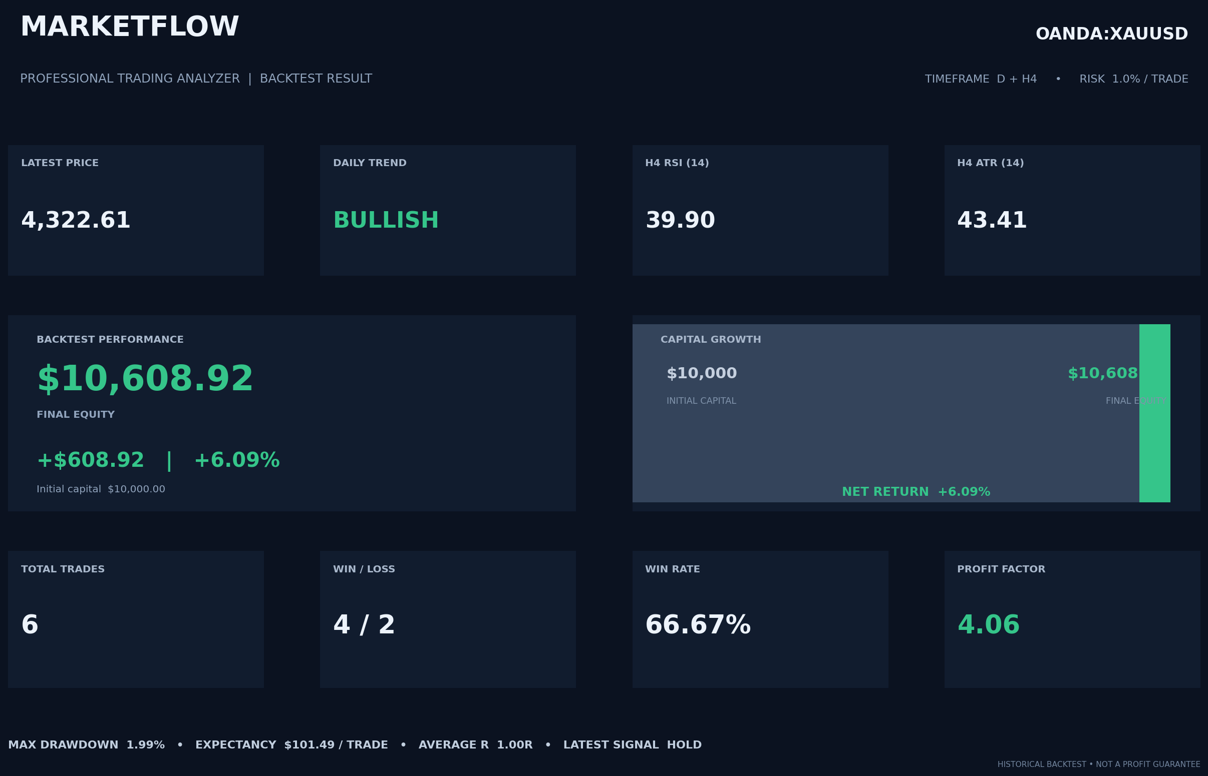
Result:
3. Results and Discussion
3.1. Market Data and Indicator Outputs
When executed successfully, the program produces Daily and H4 candle datasets for OANDA:XAUUSD and reports the number of observations retrieved for each timeframe. The normalized datasets contain OHLC values and, where supplied by the API, volume information.
The indicator-processing stage adds EMA20, EMA50, RSI14, MACD, MACD signal, MACD histogram, and ATR14 columns. The merged dataset combines the H4 observations with the latest Daily features treated as available at each H4 observation time.
The source code is designed to print the latest Daily and H4 values, the latest generated signal, and a distribution of BUY, SELL, and HOLD classifications. No execution log or numerical output is included with the uploaded source file; therefore, specific latest prices, signal counts, or indicator values cannot be reported as observed findings here.
3.2. Multi-Timeframe Trend Confirmation
The strategy uses the Daily timeframe as a directional filter and the H4 timeframe as an entry-confirmation layer. This structure is intended to prevent the system from treating every short-term price crossover as an independent trading opportunity.
The BUY and SELL rules require agreement between the Daily direction, H4 EMA structure, price crossover, RSI range, and MACD relationship. As a result, the system may produce HOLD when the market does not satisfy all required conditions. This is a rule-based filtering mechanism, not a guarantee that generated signals will be profitable.
3.3. Backtesting Outputs
The backtesting engine records trade direction, signal time, entry time, exit time, entry and exit prices, stop-loss, take-profit, ATR, position quantity, cash risk, gross PNL, commission, net PNL, R multiple, exit reason, and equity before and after each trade.
The resulting summary reports initial capital, final equity, total trades, winning and losing trades, win rate, profit factor, net PNL, total return, maximum drawdown, expectancy, and average R multiple. These outputs enable a structured evaluation of the historical behavior of the configured rules.
Because the uploaded material contains the program source rather than a verified execution report, this section does not assign numerical values to those performance measures.
3.4. Visualization and Exported Files
The system is configured to save the following visual outputs:
XAUUSD_Daily_H4_Chart.pngXAUUSD_Equity_Curve.pngXAUUSD_Drawdown.pngwhen closed trades are available
It also exports the following datasets:
XAUUSD_Daily_H4_Historical.csvXAUUSD_Backtest_Trades.csvXAUUSD_Equity_History.csvXAUUSD_Backtest_Summary.csv
These outputs support further inspection, reporting, and reproducibility. The charts show the price and equity behavior generated by the code, while the CSV files preserve the underlying records for additional analysis.
3.5. Limitations
Several limitations should be considered when interpreting the framework.
First, the historical period is fixed in the configuration to 2025. It must be updated when a different evaluation period is required.
Second, the code assumes that candle timestamps represent candle opening times and estimates availability by adding 24 hours for Daily candles and four hours for H4 candles. This assumption should be checked against the API's timestamp convention and the instrument's trading-session calendar.
Third, the backtest uses OHLC candles rather than tick-level execution data. If both stop-loss and take-profit are touched within the same candle, the current logic checks stop-loss first. This conservative ordering is a modeling choice and does not reveal the actual intrabar price path.
Fourth, slippage and commission are set to zero by default. Consequently, reported backtest performance may differ from live trading results once realistic spreads, commissions, financing costs, and execution slippage are included.
Fifth, the position-sizing calculation treats the stop distance as the cash risk per unit. Actual XAUUSD contract specifications, account currency, lot sizing, leverage, and broker-specific tick values must be incorporated before using the calculated quantity in a live account.
Finally, historical backtesting is not evidence of future profitability. Robust assessment would require out-of-sample testing, sensitivity analysis of strategy parameters, realistic trading costs, and validation across different market regimes.
4. Conclusion
This article presented MarketFlow Professional Trading Analyzer, a Python-based framework for multi-timeframe technical analysis and historical evaluation of a trend-following strategy on XAUUSD. The system retrieves Daily and H4 market data through the MarketFlow API, normalizes candle records, calculates EMA20, EMA50, RSI14, MACD, and ATR14, and combines higher-timeframe direction with H4 entry conditions.
The framework further implements ATR-based stop-loss and take-profit levels, risk-based position sizing, sequential trade simulation, and performance calculations. Its visualization and export modules produce candlestick, equity, and drawdown charts alongside historical, trade-level, equity, and summary CSV files.
The main contribution of the implementation is the integration of data acquisition, indicator processing, signal generation, risk management, backtesting, and reporting into one reproducible Python workflow. However, the framework should be regarded as an analytical and testing tool rather than a proven predictive or profitable trading system. Its results depend on API data quality, timestamp assumptions, instrument specifications, execution-cost settings, and the limitations of OHLC-based simulation.
Future development may include realistic spread and commission modeling, broker-specific contract-value calculations, tick-level or lower-timeframe execution simulation, walk-forward testing, out-of-sample validation, parameter sensitivity analysis, and automated data refresh. These extensions would strengthen the reliability and practical relevance of the framework.
References and Implementation Notes
The implementation is based on the uploaded Python source code and the MarketFlow API endpoints referenced in that source. The program requests the API usage guide, searches the market instrument, and retrieves chart-range data. No external academic references or independently verified API documentation were supplied with the source file.
Risk disclaimer: Historical backtesting does not guarantee future trading performance. This code is provided for educational and analytical purposes and should be validated against broker specifications before any live trading use.