
Financial markets are influenced by investment decisions made by individual investors, institutional investors, asset managers, and large investment organizations. Monitoring reported investor activity can provide useful information about portfolio allocation, changes in stock ownership, and investment preferences.
Institutional investment disclosures are particularly relevant because they provide information about securities held by investment managers. These disclosures can help analysts examine changes in reported portfolio positions and identify stocks receiving relatively greater investment attention.
One prominent investor frequently examined in financial market research is Warren Buffett. His investment activities are often analyzed to understand portfolio composition, capital allocation, and changes in reported equity holdings.
However, analyzing investor transactions manually can be challenging because financial disclosures are distributed across different data sources and presented in varying formats. A systematic analytical framework is therefore useful for collecting, processing, and summarizing transaction information.
Python provides an effective environment for automating these activities. Through application programming interfaces (APIs), financial datasets can be retrieved, transformed into structured tables, analyzed using numerical operations, and presented through interactive or static visualizations.
This article introduces MarketFlow Insider Trading Analyzer, a Python-based financial analytics framework developed using the MarketFlow All-in-One Market Finance API through RapidAPI.
The system retrieves investor information through the /list-investors endpoint and reported BUY and SELL transaction records through the /trade-activity endpoint.
The analysis focuses on the investor identifier warren-buffett and covers the period April 1, 2025, to July 1, 2025. Each transaction request retrieves a maximum of 100 records.
The analytical framework processes the original API responses, standardizes transaction information, calculates changes in share ownership, and aggregates transaction values by ticker symbol.
The system subsequently classifies stocks into BUY DOMINANT, SELL DOMINANT, and BALANCED categories based on the relationship between reported BUY and SELL values.
The final outputs include transaction summaries, stock-level analytics, top BUY and SELL rankings, a BUY-dominant watchlist, and an automated financial dashboard.
The primary objective is to develop a reproducible Python workflow for monitoring reported investor activity and transforming transaction records into structured financial intelligence.
Terminology note: Although the project retains its original name, Insider Trading Analyzer, the retrieved Warren Buffett portfolio activity should not automatically be interpreted as illegal insider trading or real-time transactions. The source code itself acknowledges that Form 13F filings represent reported holdings rather than real-time trades. The analysis therefore focuses on reported portfolio activity and changes in disclosed share ownership.
2. Methodology
The MarketFlow Insider Trading Analyzer is organized into five computational cells. Each cell performs a specific function within the data collection, processing, analysis, visualization, and reporting workflow.
Cell | Main function |
|---|---|
Cell 1 | Library installation, API authentication, investor configuration, and output directory. |
Cell 2 | Retrieval of investor database and BUY/SELL transaction records. |
Cell 3 | Transaction normalization, numerical conversion, share change calculation, and ticker standardization. |
Cell 4 | Transaction value aggregation, stock activity classification, and watchlist generation. |
Cell 5 | Dashboard visualization, CSV exports, and analytical report generation. |
2.1. System Configuration and API Integration
The system uses Python libraries including Requests, Pandas, NumPy, Matplotlib, JSON, and OS.
Requests handles HTTP communication with the MarketFlow API. Pandas manages structured financial datasets, NumPy supports numerical calculations, and Matplotlib generates financial visualizations.
API authentication is managed through the RapidAPI key using Python's getpass module. This prevents the API key from being directly displayed during notebook execution.
The analysis configuration specifies the investor identifier, reporting period, and transaction retrieval limit.
The output directory is named marketflow_insider_results, where the system stores processed transaction data, analytical summaries, dashboard images, and the final text report.
Code — Cell 1: Library Imports and API Configuration
# ============================================================
# MARKETFLOW INSIDER TRADING ANALYZER
# CELL 1: IMPORTS & CONFIGURATION
# ============================================================

!pip -q install requests pandas numpy matplotlib

import requests
import pandas as pd
import numpy as np
import matplotlib.pyplot as plt
import json
import os
import getpass
from datetime import datetime

# RapidAPI Configuration
API_KEY = getpass.getpass("Enter your RapidAPI Key: ")

BASE_URL = "https://marketflow-all-in-one-market-finance-api.p.rapidapi.com"

HEADERS = {
    "x-rapidapi-key": API_KEY,
    "x-rapidapi-host": "marketflow-all-in-one-market-finance-api.p.rapidapi.com"
}

# Analysis Configuration
INVESTOR_SLUG = "warren-buffett"
START_DATE = "2025-04-01"
END_DATE = "2025-07-01"

TIME_RANGE = f"{START_DATE}:{END_DATE}"
TRADE_LIMIT = 100

OUTPUT_DIR = "marketflow_insider_results"
os.makedirs(OUTPUT_DIR, exist_ok=True)

print("=" * 60)
print("MARKETFLOW INSIDER TRADING ANALYZER")
print("=" * 60)
print(f"Investor       : {INVESTOR_SLUG}")
print(f"Analysis Date  : {TIME_RANGE}")
print(f"Trade Limit    : {TRADE_LIMIT}")
print("System Status  : READY")
2.2. Investor Database and Transaction Data Collection
The second computational cell retrieves investor information and reported transaction records through three API requests.
The first request accesses /list-investors to retrieve the investor database.
The second request accesses /trade-activity with the transaction type configured as buy.
The third request accesses the same endpoint with the transaction type configured as sell.
Both transaction requests use the same investor identifier, date range, and retrieval limit to maintain consistency between the BUY and SELL datasets.
A reusable api_request() function manages HTTP communication and validates API responses. The extract_records() function extracts transaction records from commonly used JSON response structures.
The retrieved BUY and SELL records are converted into separate Pandas DataFrames and combined into a unified transaction dataset named trades_raw.
This structure allows the subsequent analytical process to evaluate transaction activity using a consistent data format.
Code — Cell 2: Full API Data Collection
# ============================================================
# CELL 2: API DATA COLLECTION
# ============================================================

def api_request(endpoint, params=None):
    url = f"{BASE_URL}/{endpoint}"

    response = requests.get(
        url,
        headers=HEADERS,
        params=params,
        timeout=30
    )

    response.raise_for_status()
    return response.json()


def extract_records(data):
    """Extract records from common API response structures."""

    if isinstance(data, list):
        return data

    if isinstance(data, dict):
        for key in ["data", "results", "trades",
                    "investors", "items", "records"]:
            if key in data:
                result = extract_records(data[key])
                if result:
                    return result

    return []


# 1. Investor Database
print("Downloading investor database...")

investor_response = api_request("list-investors")
investor_records = extract_records(investor_response)

investors_df = pd.json_normalize(investor_records)

# 2. Trade Activity: BUY
print("Downloading BUY transactions...")

buy_response = api_request(
    "trade-activity",
    params={
        "skip": 0,
        "trade_type": "buy",
        "limit": TRADE_LIMIT,
        "slug": INVESTOR_SLUG,
        "time_range": TIME_RANGE
    }
)

buy_records = extract_records(buy_response)

# 3. Trade Activity: SELL
print("Downloading SELL transactions...")

sell_response = api_request(
    "trade-activity",
    params={
        "skip": 0,
        "trade_type": "sell",
        "limit": TRADE_LIMIT,
        "slug": INVESTOR_SLUG,
        "time_range": TIME_RANGE
    }
)

sell_records = extract_records(sell_response)

# Combine transactions
buy_df = pd.json_normalize(buy_records)
sell_df = pd.json_normalize(sell_records)

buy_df["trade_type"] = "BUY"
sell_df["trade_type"] = "SELL"

trades_raw = pd.concat(
    [buy_df, sell_df],
    ignore_index=True
)

print("\nDATA COLLECTION COMPLETED")
print("-" * 50)
print("Investors retrieved :", len(investors_df))
print("BUY transactions    :", len(buy_df))
print("SELL transactions   :", len(sell_df))
print("Total transactions  :", len(trades_raw))

print("\nAvailable trade columns:")
print(trades_raw.columns.tolist())

if trades_raw.empty:
    print("\nWARNING: No transactions returned by API.")
2.3. Transaction Data Processing and Normalization
The third computational cell converts the original transaction records into a standardized analytical dataset.
The initial processing stage renames selected API fields into more readable column names. For example, the field T is converted into ticker, while trade_date becomes date.
Numerical conversion is performed on the available fields, including shares before the transaction, shares after the transaction, transaction price, transaction value, and portfolio value.
One of the main calculations is the change in share ownership:
\[ Shares\ Change = Shares\ After-Shares\ Before \]
The absolute value of this difference is then used as the transaction activity measurement:
\[ Shares = |Shares\ Change| \]
The system also converts transaction dates and filing dates into datetime formats.
Ticker symbols and transaction types are standardized into uppercase strings to ensure consistency during aggregation.
Records with missing ticker, price, or transaction value information are removed. The resulting dataset is sorted chronologically according to the transaction date.
The normalized dataset provides the foundation for calculating BUY and SELL activity, transaction values, and ticker-level portfolio changes.
Code — Cell 3: Full Data Processing and Normalization
# ============================================================
# CELL 3: DATA PROCESSING & NORMALIZATION
# ============================================================

trades = trades_raw.copy()

# Map original API fields
column_mapping = {
    "T": "ticker",
    "company": "company",
    "trade_date": "date",
    "filing_date": "filing_date"
}

trades = trades.rename(columns={
    k: v for k, v in column_mapping.items()
    if k in trades.columns
})

# Convert numeric columns
numeric_columns = [
    "shares_before",
    "shares_after",
    "price",
    "value",
    "portfolio_value"
]

for col in numeric_columns:
    if col in trades.columns:
        trades[col] = pd.to_numeric(
            trades[col], errors="coerce"
        )

# Calculate changes in share ownership
trades["shares_change"] = (
    trades["shares_after"] -
    trades["shares_before"]
)

# Use absolute share changes for activity measurement
trades["shares"] = trades["shares_change"].abs()

# Convert dates
trades["date"] = pd.to_datetime(
    trades["date"], errors="coerce"
)

trades["filing_date"] = pd.to_datetime(
    trades["filing_date"], errors="coerce"
)

# Standardize ticker
trades["ticker"] = (
    trades["ticker"]
    .astype(str)
    .str.upper()
    .str.strip()
)

# Standardize transaction type
trades["trade_type"] = (
    trades["trade_type"]
    .astype(str)
    .str.upper()
)

# Remove invalid records
trades = trades.dropna(
    subset=["ticker", "price", "value"]
)

trades = trades[
    trades["ticker"].ne("") &
    trades["ticker"].ne("NAN")
]

# Sort transactions
trades = trades.sort_values(
    "date"
).reset_index(drop=True)

print("=" * 60)
print("DATA NORMALIZATION COMPLETED")
print("=" * 60)

print("Total records :", len(trades))
print("BUY records   :", len(trades[trades["trade_type"] == "BUY"]))
print("SELL records  :", len(trades[trades["trade_type"] == "SELL"]))
print("Unique stocks :", trades["ticker"].nunique())

print("\nNORMALIZED DATA")
display(
    trades[
        [
            "ticker",
            "company",
            "trade_type",
            "shares_before",
            "shares_after",
            "shares_change",
            "price",
            "value",
            "date"
        ]
    ].head(15)
)
2.4. Trading Analytics and Stock Activity Classification
The fourth computational cell performs the primary financial analysis.
The normalized transaction dataset is divided into two groups: BUY transactions and SELL transactions.
The system calculates the total transaction value for each group:
\[ BUY\ Value = \sum BUY\ Transactions \]
\[ SELL\ Value = \sum SELL\ Transactions \]
The net transaction value is calculated as:
\[ Net\ Value = BUY\ Value-SELL\ Value \]
The same calculation is applied to share activity:
\[ Net\ Shares = BUY\ Shares-SELL\ Shares \]
These calculations provide an aggregate overview of reported transaction activity during the selected period.
The system then generates a ticker-level summary using a pivot table. Each ticker receives separate BUY and SELL transaction values.
Three additional metrics are calculated:
NET_VALUE: difference between BUY and SELL transaction values.TOTAL_ACTIVITY: combined BUY and SELL transaction values.BUY_RATIO: percentage of BUY value relative to total transaction activity.
The activity classification uses a ratio-based rule.
A stock is classified as BUY DOMINANT when its BUY value exceeds 1.5 times its SELL value. It is classified as SELL DOMINANT when its SELL value exceeds 1.5 times its BUY value. Other stocks are classified as BALANCED.
The ticker summary is subsequently sorted by net transaction value to identify stocks with relatively higher reported BUY or SELL activity.
The system generates three analytical outputs: the top ten BUY stocks, the top ten SELL stocks, and the BUY-dominant watchlist.
Code — Cell 4: Full Trading Analytics Engine
# ============================================================
# CELL 4: TRADING ANALYTICS ENGINE
# ============================================================

if trades.empty or "ticker" not in trades.columns:
    raise ValueError("No valid trade data available.")

# Separate transactions
buy_trades = trades[
    trades["trade_type"] == "BUY"
].copy()

sell_trades = trades[
    trades["trade_type"] == "SELL"
].copy()

# Transaction value
buy_value = buy_trades["value"].sum()
sell_value = sell_trades["value"].sum()

net_value = buy_value - sell_value

# Share activity
buy_shares = buy_trades["shares"].sum()
sell_shares = sell_trades["shares"].sum()

net_shares = buy_shares - sell_shares

# Transaction counts
buy_count = len(buy_trades)
sell_count = len(sell_trades)

# Ticker analytics
ticker_summary = trades.pivot_table(
    index="ticker",
    columns="trade_type",
    values="value",
    aggfunc="sum",
    fill_value=0
)

ticker_summary = ticker_summary.reindex(
    columns=["BUY", "SELL"],
    fill_value=0
)

# Calculate net activity
ticker_summary["NET_VALUE"] = (
    ticker_summary["BUY"] -
    ticker_summary["SELL"]
)

ticker_summary["TOTAL_ACTIVITY"] = (
    ticker_summary["BUY"] +
    ticker_summary["SELL"]
)

ticker_summary["BUY_RATIO"] = np.where(
    ticker_summary["TOTAL_ACTIVITY"] > 0,
    ticker_summary["BUY"] /
    ticker_summary["TOTAL_ACTIVITY"] * 100,
    0
)

# Activity classification
def classify_activity(row):

    if row["BUY"] > row["SELL"] * 1.5:
        return "BUY DOMINANT"

    elif row["SELL"] > row["BUY"] * 1.5:
        return "SELL DOMINANT"

    else:
        return "BALANCED"

ticker_summary["ACTIVITY_SIGNAL"] = (
    ticker_summary.apply(classify_activity, axis=1)
)

# Rank stocks
ticker_summary = ticker_summary.sort_values(
    "NET_VALUE",
    ascending=False
)

top_buy = ticker_summary.sort_values(
    "BUY",
    ascending=False
).head(10)

top_sell = ticker_summary.sort_values(
    "SELL",
    ascending=False
).head(10)

# Overall activity
if net_value > 0:
    market_condition = "BUY DOMINANT"

elif net_value < 0:
    market_condition = "SELL DOMINANT"

else:
    market_condition = "BALANCED"

# Generate report
print("=" * 65)
print("       MARKETFLOW TRADING INTELLIGENCE REPORT")
print("=" * 65)

print(f"Investor             : {INVESTOR_SLUG}")
print(f"Analysis Period      : {TIME_RANGE}")

print("\nTRANSACTION SUMMARY")
print("-" * 50)

print(f"Total Transactions   : {len(trades)}")
print(f"BUY Transactions     : {buy_count}")
print(f"SELL Transactions    : {sell_count}")

print("\nSHARE ACTIVITY")
print("-" * 50)

print(f"BUY Shares           : {buy_shares:,.0f}")
print(f"SELL Shares          : {sell_shares:,.0f}")
print(f"Net Shares           : {net_shares:,.0f}")

print("\nTRANSACTION VALUE")
print("-" * 50)

print(f"BUY Value            : ${buy_value:,.2f}")
print(f"SELL Value           : ${sell_value:,.2f}")
print(f"NET Activity         : ${net_value:,.2f}")

print("\nMARKET ACTIVITY")
print("-" * 50)

print(f"Market Condition     : {market_condition}")
print(f"Unique Stocks        : {trades['ticker'].nunique()}")

print("\nTOP 10 BUY STOCKS")
display(top_buy)

print("\nTOP 10 SELL STOCKS")
display(top_sell)

print("\nBUY DOMINANT WATCHLIST")

display(
    ticker_summary[
        ticker_summary["ACTIVITY_SIGNAL"] == "BUY DOMINANT"
    ].head(10)
)

print("\nANALYTICS COMPLETED SUCCESSFULLY.")
2.5. Dashboard Visualization and Data Export
The fifth computational cell transforms the analytical results into a consolidated financial dashboard.
The visualization consists of four components.
1. BUY vs SELL Transaction Value
A bar chart compares the aggregate reported BUY and SELL transaction values. This visualization provides an overview of the relative distribution of transaction activity.
2. Top 10 BUY Stocks
A horizontal bar chart displays the ten stocks with the highest aggregated BUY transaction values.
3. Top 10 SELL Stocks
A horizontal bar chart displays the ten stocks with the highest aggregated SELL transaction values.
4. Daily Transaction Activity
A time-series chart illustrates the daily distribution of BUY and SELL transaction values using the available transaction dates.
The dashboard is generated using Matplotlib with a figure size of 16 × 11 inches and a resolution of 250 DPI.
The system also exports the normalized transaction dataset, ticker-level analytics, investor database, top BUY stocks, top SELL stocks, and BUY-dominant watchlist.
Finally, a text-based report is generated to summarize investor information, transaction activity, stock rankings, and analytical observations.
Code — Cell 5: Full Dashboard, Visualization, and Export
# ============================================================
# CELL 5: DASHBOARD, VISUALIZATION & EXPORT
# ============================================================

print("=" * 65)
print("GENERATING MARKETFLOW TRADING DASHBOARD")
print("=" * 65)

# ------------------------------------------------------------
# 1. PREPARE DASHBOARD DATA
# ------------------------------------------------------------

os.makedirs(OUTPUT_DIR, exist_ok=True)

# Daily activity
daily = trades.dropna(subset=["date"]).copy()

daily["DAY"] = daily["date"].dt.strftime("%Y-%m-%d")

if not daily.empty:
    daily_activity = daily.pivot_table(
        index="DAY",
        columns="trade_type",
        values="value",
        aggfunc="sum",
        fill_value=0
    )
else:
    daily_activity = pd.DataFrame()

# ------------------------------------------------------------
# 2. CREATE DASHBOARD
# ------------------------------------------------------------

fig, axes = plt.subplots(2, 2, figsize=(16, 11))

fig.suptitle(
    "MARKETFLOW TRADING INTELLIGENCE DASHBOARD",
    fontsize=19,
    fontweight="bold"
)

# Chart 1: BUY vs SELL
axes[0, 0].bar(
    ["BUY", "SELL"],
    [buy_value, sell_value]
)

axes[0, 0].set_title("BUY vs SELL Transaction Value")
axes[0, 0].set_ylabel("Transaction Value (USD)")

# Chart 2: Top BUY Stocks
axes[0, 1].barh(
    top_buy.index.astype(str),
    top_buy["BUY"]
)

axes[0, 1].set_title("Top 10 BUY Stocks")
axes[0, 1].set_xlabel("BUY Value (USD)")
axes[0, 1].invert_yaxis()

# Chart 3: Top SELL Stocks
axes[1, 0].barh(
    top_sell.index.astype(str),
    top_sell["SELL"]
)

axes[1, 0].set_title("Top 10 SELL Stocks")
axes[1, 0].set_xlabel("SELL Value (USD)")
axes[1, 0].invert_yaxis()

# Chart 4: Daily Activity
if not daily_activity.empty:

    daily_activity.plot(
        ax=axes[1, 1],
        marker="o"
    )

    axes[1, 1].set_title("Daily Transaction Activity")
    axes[1, 1].set_ylabel("Value (USD)")
    axes[1, 1].tick_params(
        axis="x",
        rotation=45
    )

else:
    axes[1, 1].text(
        0.5, 0.5,
        "Daily data unavailable",
        ha="center",
        va="center"
    )

    axes[1, 1].set_title("Daily Transaction Activity")

plt.tight_layout(rect=[0, 0, 1, 0.95])

# Save dashboard
dashboard_path = (
    f"{OUTPUT_DIR}/marketflow_dashboard.png"
)

plt.savefig(
    dashboard_path,
    dpi=250,
    bbox_inches="tight"
)

plt.show()

# ------------------------------------------------------------
# 3. EXPORT DATASETS
# ------------------------------------------------------------

trades.to_csv(
    f"{OUTPUT_DIR}/trades_processed.csv",
    index=False
)

ticker_summary.to_csv(
    f"{OUTPUT_DIR}/ticker_analytics.csv"
)

investors_df.to_csv(
    f"{OUTPUT_DIR}/investor_database.csv",
    index=False
)

top_buy.to_csv(
    f"{OUTPUT_DIR}/top_buy_stocks.csv"
)

top_sell.to_csv(
    f"{OUTPUT_DIR}/top_sell_stocks.csv"
)

# Export watchlist
watchlist = ticker_summary[
    ticker_summary["ACTIVITY_SIGNAL"] == "BUY DOMINANT"
]

watchlist.to_csv(
    f"{OUTPUT_DIR}/stock_watchlist.csv"
)

# ------------------------------------------------------------
# 4. GENERATE ANALYSIS REPORT
# ------------------------------------------------------------

report = f"""
============================================================
       MARKETFLOW TRADING INTELLIGENCE REPORT
============================================================

INVESTOR INFORMATION
------------------------------------------------------------
Investor           : {INVESTOR_SLUG}
Requested Period   : {TIME_RANGE}

TRANSACTION SUMMARY
------------------------------------------------------------
Total Transactions : {len(trades)}
BUY Transactions   : {buy_count}
SELL Transactions  : {sell_count}
Unique Stocks      : {trades['ticker'].nunique()}

TRADING ACTIVITY
------------------------------------------------------------
BUY Value          : ${buy_value:,.2f}
SELL Value         : ${sell_value:,.2f}
NET Activity       : ${net_value:,.2f}

BUY Shares         : {buy_shares:,.0f}
SELL Shares        : {sell_shares:,.0f}
Net Shares         : {net_shares:,.0f}

MARKET CONDITION
------------------------------------------------------------
{market_condition}

TOP BUY STOCKS
------------------------------------------------------------
{top_buy.to_string()}

TOP SELL STOCKS
------------------------------------------------------------
{top_sell.to_string()}

BUY DOMINANT WATCHLIST
------------------------------------------------------------
{watchlist.to_string()}

ANALYSIS NOTES
------------------------------------------------------------
Positive net activity indicates BUY value exceeds SELL value.

Negative net activity indicates SELL value exceeds BUY value.

Activity classification is based on reported portfolio
changes and does not independently confirm future prices.

13F filings represent reported holdings, not real-time trades.

============================================================
MARKETFLOW ANALYSIS COMPLETED
============================================================
"""

report_path = (
    f"{OUTPUT_DIR}/marketflow_analysis_report.txt"
)

with open(
    report_path,
    "w",
    encoding="utf-8"
) as file:
    file.write(report)

# ------------------------------------------------------------
# 5. FINAL OUTPUT
# ------------------------------------------------------------

print("\nANALYSIS REPORT")
print(report)

print("\nEXPORTED FILES")
print("-" * 50)

for filename in sorted(os.listdir(OUTPUT_DIR)):
    filepath = os.path.join(OUTPUT_DIR, filename)

    print(
        f"{filename:<40} "
        f"{os.path.getsize(filepath):,} bytes"
    )

print("\n" + "=" * 65)
print("MARKETFLOW ANALYZER COMPLETED SUCCESSFULLY")
print("=" * 65)
Result:
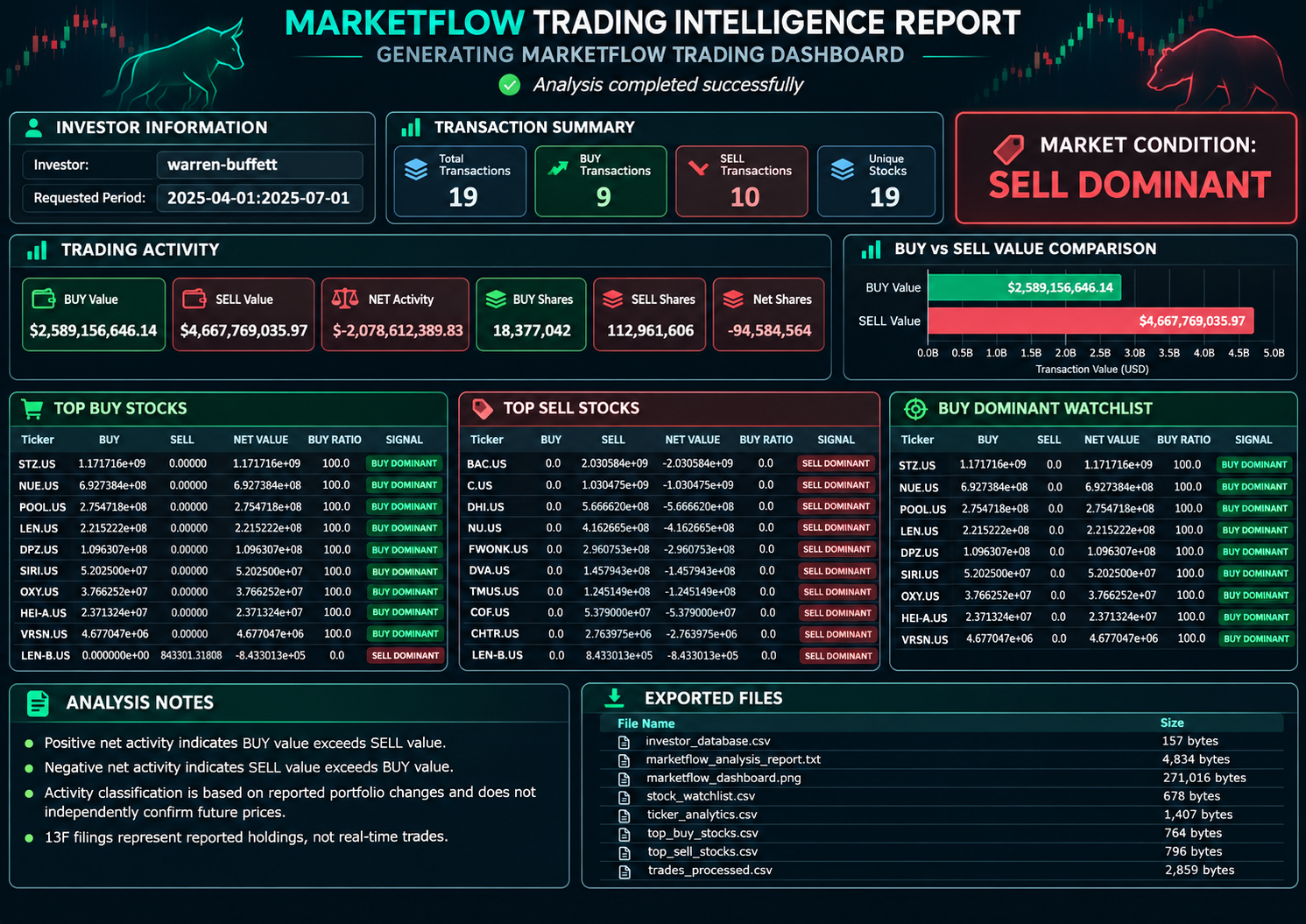
3. Results and Discussion
3.1. Investor Database and Transaction Retrieval
The data collection module retrieves investor information and reported BUY and SELL transaction records through the MarketFlow API.
The investor database provides the initial reference for identifying the selected investor. Transaction records are retrieved separately according to their transaction classifications.
The analysis focuses on the investor identifier warren-buffett, with a reporting period from April 1, 2025, to July 1, 2025.
The system combines the retrieved records into a single dataset to facilitate subsequent financial calculations.
The number of successfully retrieved records depends on API availability, endpoint permissions, and the information returned by the data provider.
3.2. Transaction Data Normalization
The normalization process transforms the original API response into a structured transaction dataset.
The main processing activities include:
Standardizing ticker symbols and transaction types.
Converting transaction values and share quantities into numerical formats.
Calculating changes in reported share ownership.
Converting transaction dates and filing dates.
Removing records with incomplete ticker, price, or transaction value information.
Sorting records chronologically.
The resulting dataset contains the information required to evaluate transaction activity across individual stocks.
The normalized dataset also allows the analytical process to distinguish BUY and SELL records consistently.
3.3. BUY and SELL Transaction Analysis
The transaction analytics engine calculates the total BUY and SELL values during the selected reporting period.
The net transaction value provides a summary of the difference between the two categories.
A positive net value indicates that the aggregate BUY value exceeds the aggregate SELL value. A negative net value indicates that the aggregate SELL value exceeds the aggregate BUY value.
The same approach is applied to the absolute changes in reported share quantities.
These measurements provide an overview of reported portfolio activity and allow analysts to compare the relative magnitude of BUY and SELL records.
However, aggregate transaction values should not automatically be interpreted as actual cash inflows or outflows because reported changes in holdings may reflect multiple portfolio activities and disclosure-related adjustments.
3.4. Stock-Level Activity Classification
The ticker analytics module evaluates BUY and SELL transaction values independently for each stock.
Each stock is assigned one of three activity classifications.
Classification | Rule | Interpretation |
|---|---|---|
BUY DOMINANT | BUY value exceeds 1.5 × SELL value | Relatively higher reported BUY activity. |
SELL DOMINANT | SELL value exceeds 1.5 × BUY value | Relatively higher reported SELL activity. |
BALANCED | Neither condition is fulfilled | BUY and SELL values do not meet the dominance threshold. |
The classification provides a systematic way to identify stocks with different reported activity patterns.
The resulting stock rankings are organized into two categories: the top ten BUY stocks and the top ten SELL stocks.
The BUY-dominant stocks are subsequently extracted into a separate watchlist for further financial examination.
3.5. Portfolio Activity and Market Condition
The overall market condition is determined by comparing aggregate BUY and SELL transaction values.
The classification consists of three possible outcomes:
BUY DOMINANT when net transaction value is positive.
SELL DOMINANT when net transaction value is negative.
BALANCED when net transaction value equals zero.
This classification provides a concise summary of the relative direction of reported transaction activity.
It does not establish whether the investor's overall portfolio performance is positive or negative, nor does it predict subsequent stock price movements.
3.6. Dashboard Visualization
The final dashboard integrates four analytical visualizations into a single financial monitoring interface.
MarketFlow Trading Intelligence Dashboard
BUY vs SELL
Comparison of aggregate transaction values.
Top 10 BUY Stocks
Stocks ranked by reported BUY value.
Top 10 SELL Stocks
Stocks ranked by reported SELL value.
Daily Transaction Activity
Daily BUY and SELL transaction values.
Dashboard components based on the original Python implementation. Actual values are generated when the notebook successfully executes.
The dashboard provides a consolidated overview of investor transaction activity and stock-level rankings.
The generated image is saved as marketflow_dashboard.png with a resolution of 250 DPI, making it suitable for inclusion in financial research reports and analytical presentations.
3.7. Exported Analytical Outputs
The system generates the following files inside the marketflow_insider_results directory.
Filename | Description |
|---|---|
| Normalized BUY and SELL transaction records. |
| Aggregated stock-level transaction analysis. |
| Retrieved investor database. |
| Top ten stocks by BUY transaction value. |
| Top ten stocks by SELL transaction value. |
| BUY-dominant stock watchlist. |
| Four-panel financial dashboard. |
| Consolidated analytical report. |
These files support further examination of reported investor activity and allow the analytical results to be used independently of the original notebook.
3.8. Limitations and Future Improvements
Several limitations should be considered when interpreting the analytical results.
First, reported portfolio holdings are not equivalent to real-time trading activity. Form 13F disclosures generally describe reportable holdings at a particular reporting date. They do not provide a complete record of every transaction executed during the reporting period.
Second, the dataset depends on API field availability. The current implementation assumes the existence of fields such as shares_before, shares_after, price, and value. Missing fields may cause processing errors and should be verified against the actual API response.
Third, the analysis uses absolute share changes. The calculation measures the magnitude of changes in reported holdings but does not independently establish the direction of every underlying transaction.
Fourth, the daily transaction visualization depends on the availability and meaning of the trade_date field. Filing dates and transaction dates should not be treated as interchangeable.
Fifth, the BUY-dominant classification uses a fixed 1.5 ratio. This threshold is a predefined analytical rule and has not been statistically validated as a predictor of future stock returns.
Future improvements could include:
Integration of historical stock prices.
Comparison of reported portfolio holdings across multiple disclosure periods.
Separation of transaction dates and filing dates.
Portfolio allocation and concentration analysis.
Sector-based investment activity analysis.
Historical performance evaluation of BUY-dominant stocks.
Risk-adjusted portfolio performance measurements.
Automated monitoring of new investor disclosures.
Integration with financial news and fundamental indicators.
These developments could expand the framework into a more comprehensive institutional investment monitoring system.
4. Conclusion
This article presents MarketFlow Insider Trading Analyzer, a Python-based financial analytics framework designed to retrieve, process, and analyze reported investor BUY and SELL activity through the MarketFlow All-in-One Market Finance API.
The system retrieves investor information and transaction records associated with Warren Buffett for the period April 1, 2025, to July 1, 2025. The analytical workflow includes API integration, JSON extraction, transaction normalization, ticker standardization, share ownership change calculations, and transaction value aggregation.
The framework further evaluates BUY and SELL transaction values at both aggregate and individual stock levels. Through a predefined ratio-based classification mechanism, stocks are categorized into BUY DOMINANT, SELL DOMINANT, and BALANCED groups.
The system also generates top BUY and SELL stock rankings, a BUY-dominant watchlist, and an overall transaction activity classification.
The visualization module combines transaction value comparisons, stock rankings, and daily transaction activity into a consolidated dashboard. The resulting datasets and reports are exported into CSV, PNG, and TXT formats to support further financial research.
Overall, MarketFlow Insider Trading Analyzer provides a practical foundation for automated investor activity monitoring using Python and financial APIs. Its integration of transaction processing, stock-level aggregation, activity classification, and dashboard visualization enables a more structured examination of reported portfolio changes.
Nevertheless, the analytical results must be interpreted within the limitations of financial disclosure data. Reported portfolio holdings do not necessarily represent real-time transactions, and BUY-dominant or SELL-dominant classifications should not be treated as independent investment recommendations.