
Introduction
broker summary broker activity data analysis Python API is a practical way to understand broker movement in the Indonesian stock market using real API data. Broker data can help traders and analysts see how transactions are distributed, which brokers are active, and which stocks have high transaction value.
In this tutorial, we will use Python in Google Colab to fetch two API datasets: Broker Activity and Broker Summary. After collecting the data, we will inspect the JSON structure, extract the available list data, convert it into DataFrames, combine both datasets, and create simple visualizations.
This article is beginner-friendly. Every cell is explained in simple language so readers can understand what the code does and why each step matters.
Cell 1 — Import Library
import requests
import pandas as pd
import matplotlib.pyplot as plt
import time
This cell imports the libraries needed for the notebook.
requests is used to fetch data from the API. pandas is used to process the data into table format. matplotlib.pyplot is used to create charts, while time is used to add a delay before making API requests.
Cell 2 — API Key Configuration
RAPIDAPI_KEY = "YOUR_RAPIDAPI_KEY_HERE"

headers = {
    "Content-Type": "application/json",
    "x-rapidapi-host": "indonesia-stock-exchange-idx.p.rapidapi.com",
    "x-rapidapi-key": RAPIDAPI_KEY
}
This cell prepares the API connection.
The RAPIDAPI_KEY is your private RapidAPI access key. The headers variable contains the information required by the API, including content type, API host, and API key.
Never publish your real API key in a public article.
Cell 3 — API URLs
broker_activity_url = "https://indonesia-stock-exchange-idx.p.rapidapi.com/api/market-detector/broker-activity/DH?limit=50&transactionType=TRANSACTION_TYPE_NET&to=2026-01-02&marketBoard=MARKET_BOARD_ALL&investorType=INVESTOR_TYPE_ALL&from=2026-01-02&page=1"

broker_summary_url = "https://indonesia-stock-exchange-idx.p.rapidapi.com/api/market-detector/broker-summary/BBCA?from=2026-01-02&transactionType=TRANSACTION_TYPE_NET&limit=25&to=2026-01-02&marketBoard=MARKET_BOARD_ALL&investorType=INVESTOR_TYPE_ALL"
This cell defines two API endpoints.
broker_activity_url is used to fetch broker activity data. In this notebook, the endpoint uses broker code DH with specific filters such as date, transaction type, market board, investor type, limit, and page.
broker_summary_url is used to fetch broker summary data for stock symbol BBCA using similar market filters.
Cell 4 — Function to Fetch API Data
def get_api_data(url):
    time.sleep(2)

    response = requests.get(url, headers=headers)

    if response.status_code == 200:
        return response.json()
    else:
        print("Gagal mengambil data:", response.status_code)
        print(response.text)
        return None
This cell creates a reusable function called get_api_data().
The function receives a URL, waits for 2 seconds using time.sleep(2), then sends a request to the API. The delay helps reduce the risk of hitting API rate limits.
If the response status code is 200, the function returns the response as JSON. If the request fails, it prints the error status and response text, then returns None.
Cell 5 — Fetch Broker Data
broker_activity_data = get_api_data(broker_activity_url)
broker_summary_data = get_api_data(broker_summary_url)
This cell fetches data from both API endpoints.
broker_activity_data stores the response from the Broker Activity API. broker_summary_data stores the response from the Broker Summary API.
At this stage, the data is still in raw JSON format.
Cell 6 — Check Data Structure
import json

print("BROKER ACTIVITY DATA:")
print(json.dumps(broker_activity_data, indent=2)[:3000])

print("\nBROKER SUMMARY DATA:")
print(json.dumps(broker_summary_data, indent=2)[:3000])
This cell checks the structure of the API responses.
The json.dumps() function formats the JSON output so it is easier to read. The [:3000] part limits the printed output to the first 3000 characters, so the notebook does not display an overly long response.
This step is important because API responses can be nested. Before converting data into a table, we need to understand where the useful list data is located.
Cell 7 — Function to Extract List Data
def cari_list_data(data, path="root"):
    if isinstance(data, list):
        print("List ditemukan di:", path)
        return data

    if isinstance(data, dict):
        for key, value in data.items():
            hasil = cari_list_data(value, path + " -> " + str(key))
            if hasil:
                return hasil

    return []
This cell creates a function named cari_list_data() to find list data inside a nested JSON response.
For beginners, a JSON response can contain many layers of dictionaries and lists. This function searches through the structure recursively. If it finds a list, it prints the path where the list was found and returns that list.
This makes the next step easier because we do not need to manually guess the exact JSON location.
Cell 8 — Process Broker Activity Data
broker_activity_list = cari_list_data(broker_activity_data)

df_activity = pd.DataFrame(broker_activity_list)
df_activity["sumber_api"] = "Broker Activity"

df_activity.head()
This cell processes the Broker Activity data.
First, it uses cari_list_data() to extract the list from broker_activity_data. Then the list is converted into a pandas DataFrame called df_activity.
A new column named sumber_api is added with the value "Broker Activity". This label helps identify where the data came from after it is combined with other data.
Finally, df_activity.head() displays the first few rows.
Cell 9 — Process Broker Summary Data
broker_summary_list = cari_list_data(broker_summary_data)

df_summary = pd.DataFrame(broker_summary_list)
df_summary["sumber_api"] = "Broker Summary"

df_summary.head()
This cell processes the Broker Summary data.
The same method is used: extract the list using cari_list_data(), convert it into a DataFrame, and add a source label.
The result is stored in df_summary, and the first few rows are displayed using df_summary.head().
Cell 10 — Check Columns
print("Jumlah data Broker Activity:", len(df_activity))
print("Kolom Broker Activity:")
print(df_activity.columns.tolist())

print("\nJumlah data Broker Summary:", len(df_summary))
print("Kolom Broker Summary:")
print(df_summary.columns.tolist())
This cell checks the number of rows and available columns in both DataFrames.
It prints:
Total Broker Activity data
Broker Activity column namesTotal Broker Summary data
Broker Summary column names
This is useful before combining and visualizing the data because we need to know which columns are available.
Cell 11 — Combine Data
df_gabungan = pd.concat([df_activity, df_summary], ignore_index=True, sort=False)

df_gabungan.head()
This cell combines Broker Activity and Broker Summary data into one DataFrame.
pd.concat() is used to merge both DataFrames vertically. The ignore_index=True parameter resets the index, while sort=False keeps the column order as much as possible.
The combined result is stored in df_gabungan.
Cell 12 — Visualize Data Count per API
jumlah_api = df_gabungan["sumber_api"].value_counts()

plt.figure(figsize=(8, 5))
jumlah_api.plot(kind="bar")
plt.title("Jumlah Data Broker Activity dan Broker Summary")
plt.xlabel("Sumber API")
plt.ylabel("Jumlah Data")
plt.xticks(rotation=0)
plt.show()
This cell creates a bar chart showing the amount of data from each API source.
The value_counts() function counts how many rows come from Broker Activity and how many come from Broker Summary.
This visualization helps compare the amount of data returned by each API.
Cell 13 — Visualize Top Broker Based on Net Value
df_gabungan["nilai_net"] = pd.to_numeric(df_gabungan["bval"], errors="coerce")

top_broker = df_gabungan.dropna(subset=["nilai_net"]).sort_values(
    "nilai_net", ascending=False
).head(10)

plt.figure(figsize=(12, 6))
plt.bar(top_broker["netbs_broker_code"].astype(str), top_broker["nilai_net"])
plt.title("Top 10 Broker Berdasarkan Net Value")
plt.xlabel("Kode Broker")
plt.ylabel("Net Value")
plt.xticks(rotation=45)
plt.show()
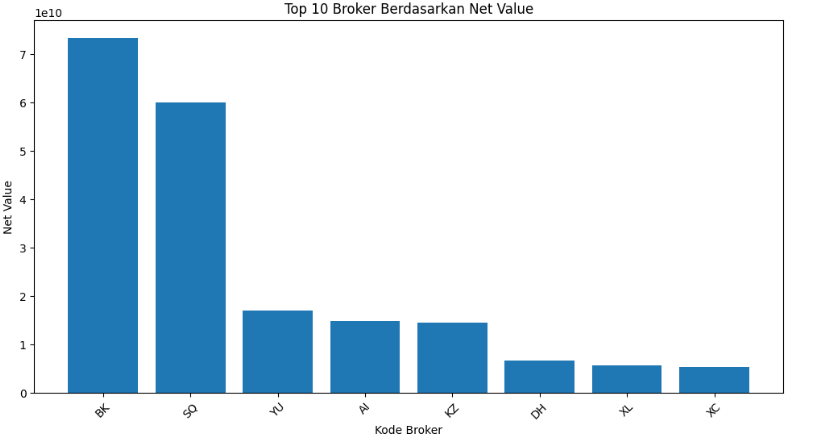
This cell analyzes the top 10 brokers based on net value.
First, the bval column is converted into numeric format and stored as nilai_net. The errors="coerce" parameter converts invalid values into missing values instead of causing an error.
Then the data is cleaned by removing rows where nilai_net is empty. After that, the data is sorted from the highest net value to the lowest, and the top 10 rows are selected.
Finally, the result is visualized as a bar chart using broker codes from netbs_broker_code.
Result :
Cell 14 — Visualize Top Stocks Based on Value
df_gabungan["nilai_value"] = pd.to_numeric(df_gabungan["bval"], errors="coerce")

top_saham = df_gabungan.dropna(subset=["nilai_value"]).sort_values(
    "nilai_value", ascending=False
).head(10)

plt.figure(figsize=(12, 6))
plt.bar(top_saham["netbs_stock_code"].astype(str), top_saham["nilai_value"])
plt.title("Top 10 Saham Berdasarkan Value")
plt.xlabel("Kode Saham")
plt.ylabel("Value")
plt.xticks(rotation=45)
plt.show()
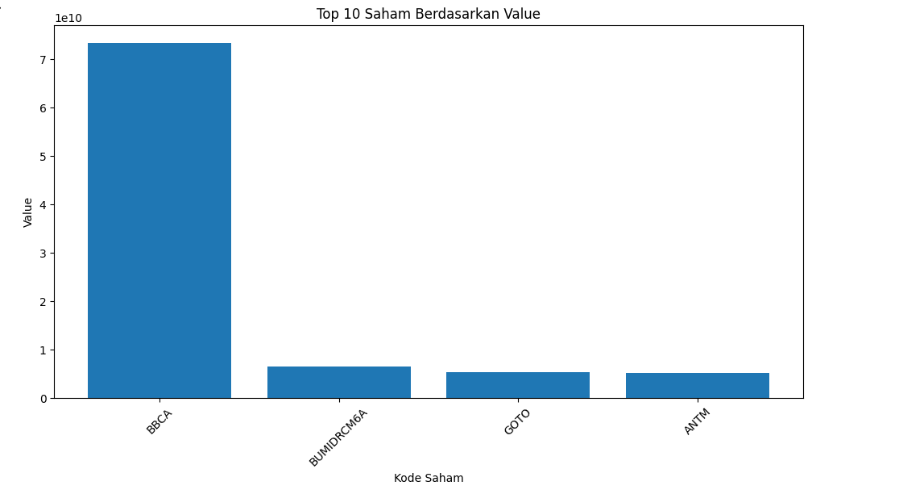
This cell analyzes the top 10 stocks based on value.
The bval column is converted into numeric format and stored as nilai_value. Then the data is sorted to find the 10 highest values.
The final chart uses netbs_stock_code as the stock code and nilai_value as the value.
For beginners, this visualization helps identify which stocks have the highest transaction value in the combined broker dataset.
Result:
Conclusion
broker summary broker activity data analysis Python API helps beginners understand broker transaction data more clearly. By using Broker Activity and Broker Summary APIs, we can collect broker-related market data, inspect the JSON structure, convert it into DataFrames, combine datasets, and visualize important patterns.
This notebook shows a complete workflow from API request to data visualization. The analysis can help identify data distribution by API source, top brokers based on net value, and top stocks based on transaction value.
The key takeaway is simple: raw broker data becomes easier to understand when it is structured into tables and visualized with charts.