Financial markets are characterized by continuous price movements, changing market trends, and varying levels of volatility. Traders need reliable analytical tools to evaluate market conditions, identify potential trading opportunities, and manage financial risks. As financial markets become increasingly data-driven, automated trading analysis systems provide an effective approach to processing historical price information and generating structured trading insights.
Technical analysis is one of the most widely used approaches in financial market evaluation. It examines historical price movements and applies mathematical indicators to identify market trends, momentum, and potential entry or exit opportunities. Indicators such as Exponential Moving Average (EMA), Relative Strength Index (RSI), Moving Average Convergence Divergence (MACD), and Average True Range (ATR) provide different perspectives on market behavior.
However, analyzing multiple indicators manually can be time-consuming and may lead to inconsistent trading decisions. Traders must collect historical price data, calculate technical indicators, compare market conditions, determine potential entry prices, and establish appropriate stop-loss and take-profit levels.
Python provides an effective environment for automating these analytical processes. Through financial APIs and data analysis libraries, Python can retrieve historical market information, calculate technical indicators, evaluate trading conditions, and generate interactive financial visualizations.
This article presents AI Trading Analyzer, a Python-based financial market analysis system developed using the MarketFlow All-in-One Market Finance API. The system integrates market discovery, historical price retrieval, technical indicator calculations, automated trading signals, and risk management into a unified analytical framework.
The implementation focuses on the BTCUSDT trading pair through Binance market data, although the instrument configuration can also be adjusted for other supported assets, including XAUUSD and EURUSD.
The analytical framework evaluates market conditions using EMA 20, EMA 50, RSI 14, MACD, and ATR. It also identifies recent support and resistance levels using a rolling 20-period calculation.
To generate trading decisions, the system combines four directional conditions: price positioning relative to EMA 20, the relationship between EMA 20 and EMA 50, MACD momentum, and RSI conditions. Each condition contributes to either a BUY or SELL score.
The system subsequently generates BUY, SELL, or WAIT classifications based on the accumulated scores. When a trading signal is identified, ATR is used to calculate the proposed stop-loss and take-profit levels according to a predefined risk-reward ratio.
In addition, the framework calculates the monetary risk based on initial trading capital and the selected risk percentage. This information is used to estimate the position size based on the distance between the entry price and stop-loss level.
The final output includes a trading analysis report, an interactive candlestick dashboard with EMA overlays, and an RSI visualization.
The primary objective of this implementation is to demonstrate how Python and financial market APIs can be integrated into an automated trading decision-support system. By combining technical analysis, signal scoring, and risk management, AI Trading Analyzer provides a structured foundation for systematic market monitoring and data-driven trading decisions.
2. Methodology
The AI Trading Analyzer framework consists of five computational cells, each responsible for a specific stage of the analytical workflow.
Cell | Main function |
|---|---|
Cell 1 | Library installation, API authentication, market configuration, and risk parameters. |
Cell 2 | Market discovery through the MarketFlow search endpoint. |
Cell 3 | Historical market data retrieval through the historical chart endpoint. |
Cell 4 | OHLC data extraction, normalization, and technical indicator calculations. |
Cell 5 | Trading signal generation, risk management, and interactive dashboard visualization. |
2.1. API Configuration and Market Selection
The system uses the MarketFlow All-in-One Market Finance API through RapidAPI as its primary financial data provider.
Authentication is managed through a RapidAPI key entered interactively using Python's getpass module. This prevents the credential from being directly displayed in the notebook.
The primary market instrument is configured as:
BINANCE:BTCUSDT
The analysis uses a daily timeframe and requests 100 historical observations.
The configuration also establishes three risk management parameters:
Initial capital: 1,000.
Risk percentage: 1%.
Risk-reward ratio: 1:2.
These parameters can be modified according to the trader's analytical requirements and account currency.
2.2. Market Discovery
The second stage retrieves market information using the /v2/search/market endpoint.
The search_market() function sends the selected instrument as a query parameter and returns the API response in JSON format.
The resulting information is displayed using Python's pprint module, allowing analysts to inspect the market search response before requesting historical price information.
This stage establishes the market discovery component of the analytical workflow.
2.3. Historical Market Data Retrieval
The third stage retrieves historical market information through the /v2/chart/historical endpoint.
The API request contains five primary parameters:
Parameter | Value |
|---|---|
range | 100 |
timeframe | D |
to | Current date |
timezone | Asia/Jakarta |
symbol | BINANCE:BTCUSDT |
The get_historical() function manages the authenticated HTTP request, applies a 30-second timeout, checks the response status, and returns the historical market data in JSON format.
The retrieved information becomes the primary dataset for subsequent technical analysis.
2.4. OHLC Data Extraction and Normalization
The fourth stage converts the raw historical API response into a structured Pandas DataFrame.
The extract_candles() function supports two general response structures:
Lists containing individual OHLC dictionaries.
TradingView-style arrays containing timestamp, open, high, low, close, and volume values.
The resulting records are normalized into standard column names.
The system then converts timestamps into datetime values and transforms OHLC fields into numeric data types.
Incomplete price records are removed before the technical indicators are calculated.
2.5. Technical Indicator Calculation
The technical analysis engine calculates five primary measurements.
Exponential Moving Average (EMA)
EMA 20 and EMA 50 are calculated using exponentially weighted moving averages.
\[ EMA_t=\alpha P_t+(1-\alpha)EMA_{t-1} \]
where:
\[ \alpha=\frac{2}{n+1} \]
EMA 20 represents a shorter-term trend measurement, while EMA 50 provides a longer-term reference.
Relative Strength Index (RSI)
RSI is calculated using exponentially weighted average gains and losses over a 14-period window.
\[ RSI=100-\frac{100}{1+RS} \]
The implementation classifies RSI values according to the following thresholds:
Above 70: Overbought.
Below 30: Oversold.
Between 30 and 70: Intermediate momentum conditions.
Moving Average Convergence Divergence (MACD)
MACD is calculated using the difference between EMA 12 and EMA 26.
\[ MACD=EMA_{12}-EMA_{26} \]
The signal line is subsequently calculated using EMA 9 of the MACD series.
The relationship between these two values provides a momentum confirmation for the trading decision.
Average True Range (ATR)
ATR measures recent market volatility using the True Range calculation.
\[ TR=\max(H-L,\ |H-PC|,\ |L-PC|) \]
Where:
\(H\) = Current high.
\(L\) = Current low.
\(PC\) = Previous closing price.
ATR 14 is calculated using an exponentially weighted average with an alpha of \(1/14\).
Support and Resistance
The system identifies recent support and resistance levels using rolling 20-period calculations.
\[ Support=\min(Low_{20}) \]
\[ Resistance=\max(High_{20}) \]
These values provide preliminary historical price references for market analysis.
2.6. Trading Signal Generation
The trading decision engine evaluates four bullish and four bearish conditions.
Indicator condition | BUY point | SELL point |
|---|---|---|
Price versus EMA 20 | Price above EMA 20 | Price below EMA 20 |
EMA relationship | EMA 20 above EMA 50 | EMA 20 below EMA 50 |
MACD | MACD above signal | MACD below signal |
RSI | RSI between 50 and 70 | RSI between 30 and 50 |
Each satisfied condition contributes one point.
The final trading classification follows these rules:
BUY when the BUY score reaches at least 3.
SELL when the SELL score reaches at least 3.
WAIT when neither condition is satisfied.
The market trend is also classified independently:
BULLISH when price is above EMA 20 and EMA 20 is above EMA 50.
BEARISH when price is below EMA 20 and EMA 20 is below EMA 50.
SIDEWAYS when neither condition is satisfied.
2.7. Risk Management and Position Sizing
The risk management module calculates the proposed stop-loss and take-profit levels using ATR.
For BUY signals:
\[ SL=Entry-(1.5\times ATR) \]
\[ TP=Entry+(3\times ATR) \]
For SELL signals:
\[ SL=Entry+(1.5\times ATR) \]
\[ TP=Entry-(3\times ATR) \]
The resulting distance establishes a nominal risk-reward ratio of 1:2.
The monetary risk is calculated as:
\[ Risk\ Money= Initial\ Capital\times\frac{Risk\ Percentage}{100} \]
The estimated position size is then calculated using:
\[ Position\ Size= \frac{Risk\ Money}{|Entry-SL|} \]
This calculation provides a preliminary position-size estimate. Actual tradable quantity must also account for contract specifications, lot sizes, leverage, exchange rules, fees, and the account's currency.
2.8. Interactive Trading Dashboard
The final stage generates two interactive financial visualizations using Plotly.
The first visualization displays historical candlestick movements with EMA 20 and EMA 50 overlays.
The second visualization presents RSI 14 with horizontal reference levels at 70 and 30.
Both visualizations use the Plotly dark theme and are designed to support interactive examination of market conditions.
3. Implementation and Full Python Code
The following implementation is based on the uploaded ai_trading_analyzer.py file. The complete program is divided into five cells, following the original notebook structure.
Cell 1 — Installation, API Configuration, and Trading Parameters
The first cell installs the required Python libraries and initializes the MarketFlow API connection.
It also defines the trading instrument, timeframe, historical data range, initial capital, risk percentage, and risk-reward ratio.
The API key is entered interactively using getpass to avoid exposing authentication credentials in the notebook.
Code — Cell 1
!pip -q install pandas numpy requests plotly ta

import requests, pandas as pd, numpy as np
import plotly.graph_objects as go
from getpass import getpass
from datetime import datetime

# API CONFIGURATION
API_KEY = getpass("Masukkan RapidAPI Key: ")
HOST = "marketflow-all-in-one-market-finance-api.p.rapidapi.com"
BASE = f"https://{HOST}"

HEADERS = {
    "x-rapidapi-key": API_KEY,
    "x-rapidapi-host": HOST
}

# TRADING CONFIGURATION
SYMBOL = "BINANCE:BTCUSDT"  # Contoh: XAUUSD, EURUSD
TIMEFRAME = "D"             # 1, 5, 15, 30, 60, D, W
RANGE = 100
TO_DATE = datetime.now().strftime("%Y-%m-%d")

INITIAL_CAPITAL = 1000
RISK_PERCENT = 1
RISK_REWARD = 2

print("TRADING ANALYZER READY")
print("Symbol:", SYMBOL)
print("Timeframe:", TIMEFRAME)
Cell 2 — Market Search API
The second cell implements the market discovery function using the /v2/search/market endpoint.
The search_market() function sends the configured trading symbol as a query parameter and retrieves the corresponding market information.
The response is displayed using pprint to make the JSON structure easier to inspect.
This stage helps verify the market instrument before retrieving its historical price data.
Code — Cell 2
def search_market(query):
    url = f"{BASE}/v2/search/market"

    response = requests.get(
        url,
        headers=HEADERS,
        params={"query": query},
        timeout=30
    )

    response.raise_for_status()
    return response.json()

market = search_market(SYMBOL)

from pprint import pprint
print("MARKET SEARCH RESULT")
pprint(market)
Cell 3 — Historical Market Data Retrieval
The third cell retrieves historical market information through the /v2/chart/historical endpoint.
The request includes the selected trading symbol, timeframe, historical range, end date, and timezone.
The get_historical() function manages the HTTP request, verifies the response status, and returns the historical data in JSON format.
The raw response is displayed to help identify the structure of the returned historical price information.
Code — Cell 3
def get_historical(symbol, timeframe="D", period=100, to=None):
    url = f"{BASE}/v2/chart/historical"

    params = {
        "range": period,
        "timeframe": timeframe,
        "to": to or TO_DATE,
        "timezone": "Asia/Jakarta",
        "symbol": symbol
    }

    response = requests.get(
        url,
        headers=HEADERS,
        params=params,
        timeout=30
    )

    response.raise_for_status()
    return response.json()

raw_data = get_historical(
    SYMBOL,
    TIMEFRAME,
    RANGE,
    TO_DATE
)

print("HISTORICAL DATA RECEIVED")
pprint(raw_data if isinstance(raw_data, dict) else raw_data[:2])
Cell 4 — Technical Analysis Engine
The fourth cell transforms historical market information into a structured OHLC DataFrame.
The extract_candles() function supports both dictionary-based candle records and TradingView-style arrays.
After data extraction, the system standardizes the column names and validates the required OHLC fields.
The technical analysis engine then calculates EMA 20, EMA 50, RSI, MACD, MACD signal, ATR, support, and resistance.
The resulting dataset provides the technical information required by the trading decision engine in the next cell.
Code — Cell 4
def extract_candles(obj):
    # Format umum: list of OHLC dictionaries
    if isinstance(obj, list) and obj and isinstance(obj[0], dict):
        return obj

    if isinstance(obj, dict):
        # Format array TradingView
        if all(k in obj for k in ["t", "o", "h", "l", "c"]):
            return [
                {"time": t, "open": o, "high": h,
                 "low": l, "close": c,
                 "volume": v if "v" in obj else 0}
                for t, o, h, l, c, v in zip(
                    obj["t"], obj["o"], obj["h"],
                    obj["l"], obj["c"],
                    obj.get("v", [0] * len(obj["t"]))
                )
            ]

        for key in ["data", "result", "candles", "history", "bars"]:
            if key in obj:
                result = extract_candles(obj[key])
                if result:
                    return result

        for value in obj.values():
            result = extract_candles(value)
            if result:
                return result

    return None


candles = extract_candles(raw_data)

if not candles:
    raise ValueError(
        "Format historical belum dikenali. "
        "Periksa struktur raw_data pada Cell 3."
    )

df = pd.DataFrame(candles)

# Normalisasi nama kolom
df.columns = [str(c).lower() for c in df.columns]

aliases = {
    "time": ["time", "timestamp", "date", "datetime", "t"],
    "open": ["open", "o"],
    "high": ["high", "h"],
    "low": ["low", "l"],
    "close": ["close", "c"],
    "volume": ["volume", "vol", "v"]
}

for target, names in aliases.items():
    if target not in df.columns:
        source = next((n for n in names if n in df.columns), None)
        if source:
            df.rename(columns={source: target}, inplace=True)

required = ["open", "high", "low", "close"]
if not all(c in df.columns for c in required):
    raise ValueError(f"Kolom OHLC tidak lengkap: {df.columns.tolist()}")

if "time" in df.columns:
    if pd.api.types.is_numeric_dtype(df["time"]):
        unit = "ms" if df["time"].max() > 1e11 else "s"
        df["time"] = pd.to_datetime(df["time"], unit=unit)
    else:
        df["time"] = pd.to_datetime(df["time"])
    df = df.sort_values("time").set_index("time")

for c in required:
    df[c] = pd.to_numeric(df[c], errors="coerce")

df = df.dropna(subset=required)

# INDICATORS
df["EMA20"] = df.close.ewm(span=20, adjust=False).mean()
df["EMA50"] = df.close.ewm(span=50, adjust=False).mean()

delta = df.close.diff()
gain = delta.clip(lower=0)
loss = -delta.clip(upper=0)

avg_gain = gain.ewm(alpha=1/14, adjust=False).mean()
avg_loss = loss.ewm(alpha=1/14, adjust=False).mean()

rs = avg_gain / avg_loss.replace(0, np.nan)
df["RSI"] = 100 - (100 / (1 + rs))
df.loc[avg_loss.eq(0) & avg_gain.gt(0), "RSI"] = 100
df.loc[avg_gain.eq(0) & avg_loss.eq(0), "RSI"] = 50

ema12 = df.close.ewm(span=12, adjust=False).mean()
ema26 = df.close.ewm(span=26, adjust=False).mean()

df["MACD"] = ema12 - ema26
df["SIGNAL"] = df.MACD.ewm(span=9, adjust=False).mean()

prev_close = df.close.shift()
tr = pd.concat([
    df.high - df.low,
    (df.high - prev_close).abs(),
    (df.low - prev_close).abs()
], axis=1).max(axis=1)

df["ATR"] = tr.ewm(alpha=1/14, adjust=False).mean()

# SUPPORT & RESISTANCE
df["SUPPORT"] = df.low.rolling(20).min()
df["RESISTANCE"] = df.high.rolling(20).max()

print("TECHNICAL ANALYSIS COMPLETED")
print(df.tail(5).round(4))
Cell 5 — Trading Decision, Risk Management, and Dashboard
The fifth cell integrates all calculated indicators into the final trading decision engine.
The system evaluates the latest market observation and generates independent BUY and SELL scores.
When either score reaches at least three points, the corresponding trading signal is generated.
The ATR value determines the proposed stop-loss and take-profit distances, while the configured initial capital and risk percentage determine the monetary risk.
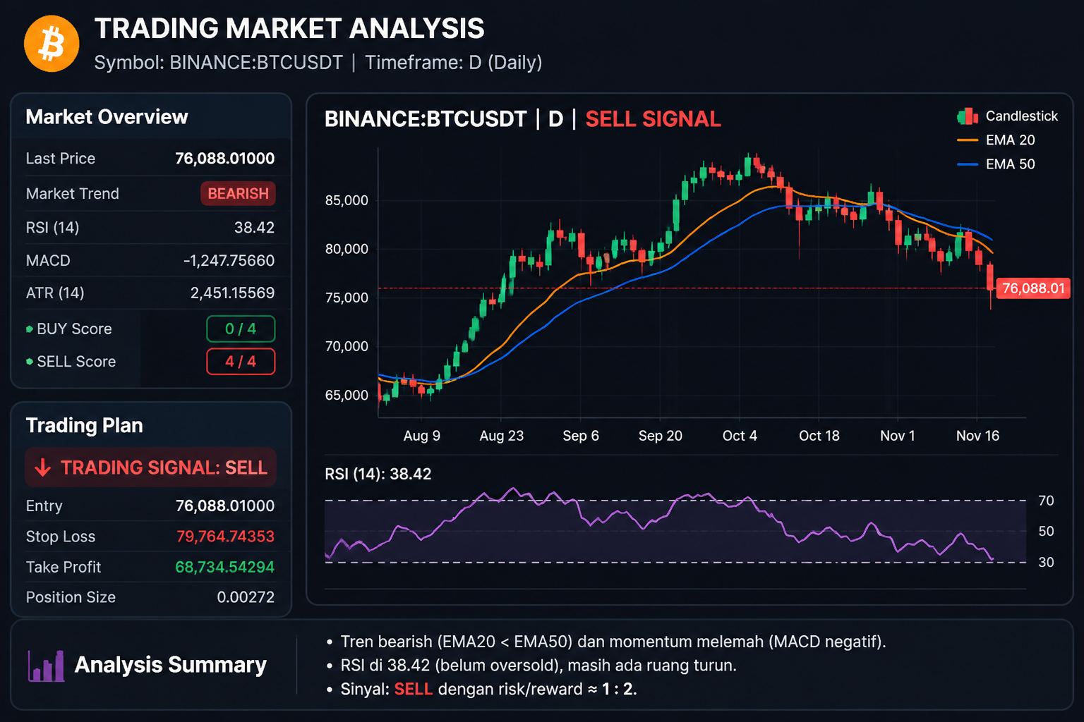
The final output includes the trading symbol, latest price, market trend, technical indicator values, BUY and SELL scores, trading signal, entry price, stop-loss, take-profit, and estimated position size.
The cell also generates an interactive candlestick dashboard with EMA 20 and EMA 50 overlays, followed by a separate RSI chart.
Code — Cell 5
last = df.iloc[-1]

price = last.close
ema20 = last.EMA20
ema50 = last.EMA50
rsi = last.RSI
macd = last.MACD
signal = last.SIGNAL
atr = last.ATR

# TREND ANALYSIS
if price > ema20 > ema50:
    trend = "BULLISH"
elif price < ema20 < ema50:
    trend = "BEARISH"
else:
    trend = "SIDEWAYS"

# SCORING
buy_score = sum([
    price > ema20,
    ema20 > ema50,
    macd > signal,
    50 < rsi < 70
])

sell_score = sum([
    price < ema20,
    ema20 < ema50,
    macd < signal,
    30 < rsi < 50
])

if buy_score >= 3:
    action = "BUY"
    entry = price
    sl = entry - 1.5 * atr
    tp = entry + 3 * atr
elif sell_score >= 3:
    action = "SELL"
    entry = price
    sl = entry + 1.5 * atr
    tp = entry - 3 * atr
else:
    action = "WAIT"
    entry = sl = tp = np.nan

# RISK MANAGEMENT
risk_money = INITIAL_CAPITAL * RISK_PERCENT / 100
risk_distance = abs(entry - sl) if action != "WAIT" else np.nan
position_size = risk_money / risk_distance if risk_distance > 0 else np.nan

print("=" * 45)
print("       TRADING MARKET ANALYSIS")
print("=" * 45)
print(f"Symbol          : {SYMBOL}")
print(f"Last Price      : {price:.5f}")
print(f"Market Trend    : {trend}")
print(f"RSI             : {rsi:.2f}")
print(f"MACD            : {macd:.5f}")
print(f"ATR             : {atr:.5f}")
print(f"BUY SCORE       : {buy_score}/4")
print(f"SELL SCORE      : {sell_score}/4")
print("-" * 45)
print(f"TRADING SIGNAL  : {action}")
print(f"ENTRY           : {entry:.5f}" if action != "WAIT" else "ENTRY : -")
print(f"STOP LOSS       : {sl:.5f}" if action != "WAIT" else "STOP LOSS : -")
print(f"TAKE PROFIT     : {tp:.5f}" if action != "WAIT" else "TAKE PROFIT : -")
print(f"POSITION SIZE   : {position_size:.5f}" if action != "WAIT" else "POSITION SIZE : -")
print("=" * 45)

# CANDLESTICK DASHBOARD
fig = go.Figure()

fig.add_trace(go.Candlestick(
    x=df.index,
    open=df.open,
    high=df.high,
    low=df.low,
    close=df.close,
    name="Candlestick"
))

fig.add_trace(go.Scatter(
    x=df.index, y=df.EMA20,
    name="EMA 20", line=dict(color="orange")
))

fig.add_trace(go.Scatter(
    x=df.index, y=df.EMA50,
    name="EMA 50", line=dict(color="blue")
))

fig.update_layout(
    title=f"{SYMBOL} | {TIMEFRAME} | {action} SIGNAL",
    template="plotly_dark",
    height=700,
    xaxis_rangeslider_visible=False
)

fig.show()

# RSI CHART
fig2 = go.Figure()
fig2.add_trace(go.Scatter(x=df.index, y=df.RSI, name="RSI 14"))
fig2.add_hline(y=70, line_dash="dash")
fig2.add_hline(y=30, line_dash="dash")
fig2.update_layout(
    title="Relative Strength Index",
    template="plotly_dark",
    height=300
)
fig2.show()
Result:
4. Results and Discussion
4.1. Market Discovery and Historical Data Retrieval
The market discovery module establishes the selected trading instrument through the MarketFlow search endpoint.
For the default configuration, the system analyzes BTCUSDT using Binance market data.
The historical data retrieval module subsequently collects 100 daily observations containing OHLC information.
The retrieved data provides the foundation for calculating technical indicators and evaluating market conditions.
The use of a configurable symbol also allows the framework to be adapted to other supported financial instruments by changing the SYMBOL parameter.
4.2. Technical Indicator Analysis
The technical analysis engine combines EMA, RSI, MACD, and ATR to evaluate different dimensions of market behavior.
EMA 20 and EMA 50 provide information about trend direction and the relative positioning of short-term and medium-term price averages.
RSI 14 evaluates momentum conditions and identifies intermediate, overbought, and oversold readings.
MACD provides additional momentum confirmation through the relationship between its main line and signal line.
ATR measures recent price volatility and becomes the basis for calculating stop-loss and take-profit distances.
The combination of these indicators provides a more structured analytical perspective than relying on a single technical measurement.
4.3. Automated Trading Signal Generation
The trading decision engine evaluates four conditions for BUY and SELL signals.
Each satisfied condition contributes one point to the corresponding score.
The system generates a BUY signal when at least three bullish conditions are satisfied. Similarly, a SELL signal is generated when at least three bearish conditions are satisfied.
When neither score reaches the required threshold, the system produces a WAIT classification.
This approach provides a straightforward mechanism for combining multiple technical confirmations into a single trading decision.
However, the score is a rule-based indicator confirmation, not a statistical probability of a successful trade.
4.4. ATR-Based Stop-Loss and Take-Profit Calculation
The risk management module uses ATR to determine the distance between the entry price and the proposed stop-loss and take-profit levels.
For BUY signals, the stop-loss is positioned below the entry price, while the take-profit is positioned above it.
For SELL signals, the opposite arrangement is applied.
The implementation uses a stop-loss distance of 1.5 ATR and a take-profit distance of 3 ATR.
This creates a nominal risk-reward ratio of 1:2.
The resulting levels provide a systematic reference for evaluating potential trade exposure.
Nevertheless, ATR-based levels do not guarantee that a position will close at the intended price, particularly during periods of high volatility or market gaps.
4.5. Position Sizing and Capital Risk Evaluation
The position sizing module calculates the monetary risk using the initial capital and selected risk percentage.
With the default configuration, the system allocates 1% of the initial capital as the nominal risk budget for a trade.
The estimated position size is calculated by dividing this monetary risk by the distance between the entry price and stop-loss.
This approach helps establish a consistent relationship between account capital and the potential loss associated with a trade.
However, the current implementation produces a simplified position-size estimate. It does not automatically account for contract multipliers, exchange lot sizes, leverage, commissions, funding costs, or slippage.
Consequently, the calculated quantity must be adjusted to the actual specifications of the selected trading instrument before execution.
4.6. Interactive Candlestick Dashboard
The candlestick dashboard provides a visual representation of historical price movements.
The visualization includes:
Historical candlestick prices.
EMA 20.
EMA 50.
Trading symbol.
Timeframe.
Generated trading signal in the chart title.
The EMA overlays allow traders to observe the relationship between price movements and moving average trends.
The interactive Plotly interface also enables users to inspect historical observations and examine different sections of the price chart.
4.7. RSI Visualization
The RSI chart presents the calculated momentum values across the historical observation period.
Two horizontal reference lines are displayed at 70 and 30.
These reference levels help identify periods when the RSI enters traditionally overbought or oversold conditions.
The visualization complements the candlestick dashboard by providing a separate view of market momentum.
Together, the two visualizations offer a more comprehensive overview of the technical conditions used by the trading decision engine.
4.8. Limitations and Future Improvements
Several limitations should be considered when interpreting the analytical results.
First, the trading signals are based on predefined rules. The BUY and SELL scores use four conditions with equal weighting. They have not been statistically validated through historical backtesting.
Second, the current framework does not include volume-based analysis. Trading volume could provide additional information about the strength of price movements and potential breakouts.
Third, the support and resistance indicators are calculated but are not directly incorporated into the trading scoring mechanism. Future development could use these levels to improve entry selection and evaluate potential price targets.
Fourth, the RISK_REWARD parameter is declared but is not directly used in the take-profit calculation. The current implementation uses fixed distances of 1.5 ATR for stop-loss and 3 ATR for take-profit, which produces a 1:2 ratio.
Fifth, the position sizing calculation is simplified. Actual trading quantity requires additional consideration of contract specifications, minimum order sizes, account currency, and transaction costs.
Sixth, the system does not include historical backtesting or performance evaluation. Therefore, its trading signals cannot yet be considered proven profitable.
Future improvements could include:
Historical strategy backtesting.
Bollinger Bands and volume analysis.
Automated support and resistance detection.
Dynamic risk-reward configuration.
Trading performance statistics.
Maximum drawdown and win-rate calculations.
Multi-asset portfolio analysis.
Automated trading alerts.
These developments could transform the current framework into a more comprehensive quantitative trading analysis platform.
5. Conclusion
AI Trading Analyzer demonstrates how Python and the MarketFlow All-in-One Market Finance API can be integrated into an automated financial market analysis system.
The framework retrieves market information, collects historical price observations, processes OHLC data, and calculates EMA 20, EMA 50, RSI, MACD, ATR, support, and resistance.
Its trading decision engine combines four technical conditions to generate BUY, SELL, or WAIT classifications.
The risk management component further calculates proposed entry prices, stop-loss levels, take-profit levels, and estimated position sizes using predefined capital and volatility parameters.
The final dashboard presents interactive candlestick charts with EMA overlays and a separate RSI visualization, allowing traders to examine historical price behavior and technical momentum.
Overall, AI Trading Analyzer provides a structured foundation for automated technical analysis and rule-based trading decision support.
Nevertheless, the generated trading signals should not be interpreted as guaranteed predictions or automatic recommendations to execute transactions. Their reliability requires further evaluation through historical backtesting, transaction-cost analysis, and real-market validation.
Future improvements involving advanced indicators, volume analysis, dynamic risk management, and portfolio-level evaluation could enhance the system's analytical capabilities.